Laboratory 8: Solution of the Quasi-geostrophic Equations
Lin Yang & John M. Stockie
List of Problems
Problem 1: Discretization of the Jacobian term
Problem 2: Numerical instability in the “straightforward” Jacobian
Problem 3: Implement the SOR relaxation
Problem 4: No-slip boundary conditions
Problem 5: Starting values for the time integration
Problem 6: Duplication of classical results
Goals
This lab is an introduction to the use of implicit schemes for the solution of PDE’s, using as an example the quasi-geostrophic equations that govern the large-scale circulation of the oceans.
You will see that the discretization of the governing equations leads to a large, sparse system of linear equations. The resulting matrix problem is solved with relaxation methods, one of which you will write the code for, by modifying the simpler Jacobi relaxation. There are two types of boundary conditions typically used for this problem, one of which you will program yourself – your computations are easily compared to previously-obtained “classical” results.
Learning Objectives
After reading and working through this lab you will be able to: * Explain one reason why one may need to solve a large system of linear equations even though the underlying method is explicit * Describe the relaxation method * Rescale a partial-differential equation * Write down the center difference approximation for the Laplacian operator * Describe what a ghost point is
Readings
There are no required readings for this lab. If you would like some additional background beyond the material in the lab itself, then you may refer to the references listed below:
Equations of motion:
Pedlosky Sections 4.6 & 4.11 (derivation of QG equations)
Nonlinear instability:
Mesinger & Arakawa (classic paper with description of instability and aliasing)
Arakawa & Lamb (non-linear instability in the QG equations, with the Arakawa-Jacobian)
Numerical methods:
Strang (analysis of implicit schemes)
McCalpin (QGbox model)
Classical numerical results:
Veronis (numerical results)
Bryan (numerical results)
[3]:
import context
from IPython.display import Image
# import the quiz script
from numlabs.lab8 import quiz8 as quiz
Introduction
An important aspect in the study of large-scale circulation in the ocean is the response of the ocean to wind stress. Solution of this problem using the full Navier-Stokes equations is quite complicated, and it is natural to look for some way to simplify the governing equations. A common simplification in many models of large-scale, wind-driven ocean circulation, is to assume a system that is homogeneous and barotropic.
It is now natural to ask:
Does the simplified model capture the important dynamics in the real ocean?
This question can be investigated by solving the equations numerically, and comparing the results to observations in the real ocean. Many numerical results are already available, and so the purpose of this lab is to introduce you to the numerical methods used to solve this problem, and to compare the computed results to those from some classical papers on numerical ocean simulations.
Some of the numerical details (in Sections Right Hand Side, Boundary Conditions, Matrix Form of Discrete Equations, Solution of the Poisson Equation by Relaxation and the appendices) are quite technical, and may be passed over the first time you read through the lab. You can get a general idea of the basic solution procedure without them. However, you should return to them later and understand the material contained in them, since these sections contain techniques that are commonly encountered when solving PDE’s, and an understanding of these sections is required for you to answer the problems in the Lab.
The Quasi-Geostrophic Model
Consider a rectangular ocean with a flat bottom, as pictured in Figure Model Ocean, and ignore curvature effects, by confining the region of interest to a mid-latitude :math:`beta`-plane.
[4]:
Image(filename='images/rect.png',width='45%')
[4]:
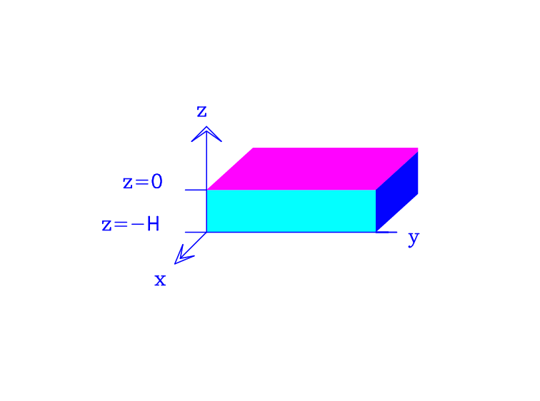
Figure Model Ocean The rectangular ocean with flat bottom, ignoring curvature effects.
More information on what is a \(\beta\)-plane and on the neglect of curvature terms in the \(\beta\)-plane approximation is given in the appendix.
If we assume that the ocean is homogeneous (it has constant density throughout), then the equations governing the fluid motion on the \(\beta\)-plane are:
(X-Momentum Eqn)
\begin{equation} \frac{\partial u}{\partial t} + u \frac {\partial u}{\partial x} + v \frac {\partial u}{\partial y} + w \frac{\partial u}{\partial z} - fv = - \, \frac{1}{\rho} \, \frac {\partial p}{\partial x} + A_v \, \frac{\partial^2 u}{\partial z^2} + A_h \, \nabla^2 u \end{equation}
(Y-Momentum Eqn)
\begin{equation} \frac{\partial v}{\partial t} + u \frac{\partial v}{\partial x} + v \frac{\partial v}{\partial y} + w \frac{\partial v}{\partial z} + fu = - \, \frac{1}{\rho} \, \frac{\partial p}{\partial y} + A_v \, \frac{\partial^2 v}{\partial z^2} + A_h \, \nabla^2 v \end{equation}
(Hydrostatic Eqn)
\begin{equation} \frac{\partial p}{\partial z} = - \rho g \end{equation}
(Continuity Eqn)
\begin{equation} \frac {\partial u}{\partial x} + \frac{\partial v}{\partial y} = - \, \frac{\partial w}{\partial z} \end{equation}
where
(X-Momentum Eqn) and (Y-Momentum Eqn) are the lateral momentum equations,
(Hydrostatic Eqn) is the hydrostatic balance (and replaces the vertical momentum equation), and
(Continuity Eqn) is the continuity (or incompressibility or conservation of volume) condition.
The variables and parameters appearing above are:
\((u,v,w)\), the fluid velocity components;
\(f(y)\), the Coriolis parameter (assumed to be a linear function of \(y\));
\(\rho\), the density (assumed constant for a homogeneous fluid);
\(A_v\) and \(A_h\), the vertical and horizontal coefficients of viscosity, respectively (constants);
\(g\), the gravitational acceleration (constant).
Equations (X-Momentum Eqn), (Y-Momentum Eqn), (Hydrostatic Eqn) and (Continuity Eqn) form a non-linear system of PDE’s, for which there are many numerical methods available. However, due to the complexity of the equations, the methods themselves are very complex, and consume a large amount of CPU time. It is therefore advantageous for us to reduce the equations to a simpler form, for which common, and more efficient numerical solution techniques can be used.
By applying a sequence of physically-motivated approximations (see Appendix Simplification of the QG Model Equations) and by using the boundary conditions, the system(X-Momentum Eqn), (Y-Momentum Eqn), (Hydrostatic Eqn) and (Continuity Eqn) can be reduced to a single PDE:
(Quasi-Geotrophic Eqn)
where
\(\psi\) is the stream function, defined by
\[u = - \frac{\partial \psi}{\partial y},\]\[v = \frac{\partial \psi}{\partial x}\]- \[\nabla_h = \left(\frac{\partial}{\partial x},\frac{\partial}{\partial y}\right)\]
is the “horizontal” gradient operator, so-called because it involves only derivatives in \(x\) and \(y\);
- \[{\cal J} (a,b) = \frac{\partial a}{\partial x} \frac{\partial b}{\partial y} - \frac{\partial a}{\partial y} \frac{\partial b}{\partial x}\]is the Jacobian operator;
\(\vec{\tau}(x,y) = \left(\,\tau_1(x,y),\tau_2(x,y)\,\right)\) is the wind stress boundary condition at the surface \(z=0\). A simple form of the wind stress might assume an ocean “box” that extends from near the equator to a latitude of about \(60^\circ\), for which typical winds are easterly near the equator and turn westerly at middle latitudes. A simple function describing this is
\[\vec{\tau} = \tau_{max} (-\cos y, 0),\]which is what we will use in this lab.
More complicated wind stress functions are possible. See McCalpin’s QGBOX documentation [p. 24] for another example.
\(\beta = df/dy\) is a constant, where \(f(y) = f_0+\beta y\) (see Appendix Definition of the Beta-plane);
\(\kappa = {1}/{H} \left[ (A_v f_0)/{2} \right]^{1/2}\) is the bottom friction scaling (constant); and
\(H\) is the vertical depth of the water column (constant).
Notice that the original (second order) system of four equations in four unknowns (\(u\), \(v\), \(w\), \(p\)) has now been reduced to a single (fourth order) PDE in one unknown function, \(\psi\). It will become clear in the next section just how much simpler the system of equations has become …
Before going on, though, we need to close the system with the boundary conditions for the stream function \(\psi\). We must actually consider two cases, based on whether or not the lateral eddy viscosity parameter, \(A_h\), is zero:
if :math:`A_h=0`: the boundary conditions are free-slip; that is, \(\psi=0\) on the boundary.
if :math:`A_hneq 0`: the boundary conditions are no-slip; that is both \(\psi\) and its normal derivative \(\nabla\psi\cdot\hat{n}\) are zero on the boundary (where \(\hat{n}\) is the normal vector to the boundary).
Scaling the Equations of Motion
In physical problems, it is not uncommon for some of the quantities of interest to differ in size by many orders of magnitude. This is of particular concern when computing numerical solutions to such problems, since then round-off errors can begin to pollute the computations (see Lab 2).
This is also the case for the QG equations, where the parameters have a large variation in size. The QG model parameters, and typical numerical values, are given in Table of Parameters. For such problems it is customary to rescale the variables in such a way that the size differences are minimized.
Problem Parameters
Symbol |
Name |
Range of Magnitude |
Units |
|---|---|---|---|
\(R\) |
Earth’s radius |
\(6.4 \times 10^6\) |
\(m\) |
\(\Omega\) |
Angular frequency for Earth |
\(7.27 \times 10^{-5}\) |
\(s^{-1}\) |
\(H\) |
Depth of active layer |
\(100 \rightarrow 4000\) |
\(m\) |
\(B\) |
Length and width of ocean |
\(1.0 \rightarrow 5.0 \times 10^6\) |
\(m\) |
\(\rho\) |
Density of water |
\(10^3\) |
\(kg/m^3\) |
\(A_h\) |
Lateral eddy viscosity |
\(0\) or \(10^1 \rightarrow 10^4\) |
\(m^2/s\) |
\(A_v\) |
Vertical eddy viscosity |
\(10^{-4} \rightarrow 10^{-1}\) |
\(m^2/s\) |
\(\tau_{max}\) |
Maximum wind stress |
\(10^{-2} \rightarrow 1\) |
\(kg m^{-1} s^{-2}\) |
\(\theta_0\) |
Latitude |
\(0 \rightarrow \frac{\pi}{3}\) |
Derived Quantities
Symbol |
Name |
Range of Magnitude |
Units |
|---|---|---|---|
\(\beta\) |
\(\beta =2\Omega \cos \theta_0 / R\) |
\(1.1 \rightarrow 2.3 \times 10^{-11}\) |
\(m^{-1} s^{-1}\) |
\(f_0\) |
\(f_0 = 2 \Omega \sin \theta_0\) |
\(0.0 \rightarrow 1.3 \times 10^{-4}\) |
\(s^{-1}\) |
\(U_0\) |
Velocity scale = \(\tau_{max}/(\beta\rho H B)\) |
\(10^{-5} \rightarrow 10^{-1}\) |
\(m s^{-1}\) |
\(\kappa\) |
bottom friction parameter |
\(0.0 \rightarrow 10^{-5}\) |
\(m^2 s^{-2}\) |
Non-dimensional Quantities
Symbol / Name |
Range of Magnitude for Quantity |
|---|---|
\(\epsilon\) / Vorticity ratio = \(U_0/(\beta B^2)\) |
(computed) |
\(\frac{\tau_{max}}{\epsilon\beta^2 \rho H B^3}\) |
\(10^{-12} \rightarrow 10^{-14}\) |
\(\frac{\kappa}{\beta B}\) |
\(4 \times 10^{-4} \rightarrow 6 \times 10^1\) |
\(\frac{A_h}{\beta B^3}\) |
\(10^{-7} \rightarrow 10^{-4}\) |
Table of Parameters
Let us go through this scaling process for the evolution equation (Quasi-Geostrophic Eqn) for the stream function, which is reproduced here for easy comparison:
The basic idea is to find typical scales of motion, and then redefine the dependent and independent variables in terms of these scales to obtain dimensionless variables.
For example, the basin width and length, \(B\), can be used as a scale for the dependent variables \(x\) and \(y\). Then, we define dimensionless variables
(x-scale eqn)
(y-scale eqn)
Notice that where \(x\) and \(y\) varied between 0 and \(B\) (where \(B\) could be on the order of hundreds of kilometres), the new variables \(x^\prime\) and \(y^\prime\) now vary between 0 and 1 (and so the ocean is now a unit square).
Similarly, we can redefine the remaining variables in the problem as
(t-scale eqn)
(\(\psi\)-scale eqn)
(\(\tau\)-scale eqn)
where the scales have been specially chosen to represent typical sizes of the variables. Here, the parameter \(\epsilon\) is a measure of the the ratio between the “relative vorticity” (\(\max|\nabla_h^2 \psi|\)) and the planetary vorticity (given by \(\beta B\)).
Now, we need only substitute for the original variables in the equations, and replace derivatives with their dimensionless counterparts; for example, using the chain rule,
Then the equation of motion becomes
(Rescaled Quasi-Geostrophic Eqn)
The superscript “\(\,^\prime\)” on \(\nabla_h\) and \({\cal J}\) signify that the derivatives are taken with respect to the dimensionless variables. Notice that each term in (Rescaled Quasi-Geostrophic Eqn) is now dimensionless, and that there are now 4 dimensionless combinations of parameters
These four expressions define four new dimensionless parameters that replace the original (unscaled) parameters in the problem.
The terms in the equation now involve the dimensionless stream function, \(\psi^\prime\), and its derivatives, which have been scaled so that they are now of order 1 in magnitude. The differences in sizes between terms in the equation are now embodied solely in the four dimensionless parameters. A term which is multiplied by a small parameter is thus truly small in comparison to the other terms, and hence additive round-off errors will not contribute substantially to a numerical solution based on this form of the equations.
For the remainder of this lab, we will use the scaled version of the equations. Consequently, the notation will be simplified by dropping the “primes” on the dimensionless variables. But, do not forget, that any solution (numerical or analytical) from the scaled equations must be converted back into dimensional variables using the scale equations.
Discretization of the QG equations
At first glance, it is probably not clear how one might discretize the QG equation (Rescaled Quasi-Geostrophic Eqn) from the previous section. This equation is an evolution equation for \(\nabla_h^2 \psi\) (the Laplacian of the stream function) but has a right hand side that depends not only on \(\nabla_h^2 \psi\), but also on \(\psi\) and \(\nabla_h^4 \psi\). The problem may be written in a more suggestive form, by letting \(\chi = \partial\psi/\partial t\). Then, the (Rescaled Quasi-Geostrophic Eqn) becomes
(Poisson Eqn)
where \(F(x,y,t)\) contains all of the terms except the time derivative. We will see that the discrete version of this equation is easily solved for the new unknown variable \(\chi\), after which
may be used to evolve the stream function in time.
The next two sections discuss the spatial and temporal discretization, including some details related to the right hand side, the boundary conditions, and the iterative scheme for solving the large sparse system of equations that arises from the Poisson equation for \(\chi\). Following that is an summary of the steps in the solution procedure.
Spatial Discretization
Assume that we are dealing with a square ocean, with dimensions \(1\times 1\) (in non-dimensional coordinates) and begin by dividing the domain into a grid of discrete points
where \(\Delta x = 1/M\) and \(\Delta y = 1/N\). In order to simplify the discrete equations, it will be helpful to assume that \(M=N\), so that \(\Delta x = \Delta y \equiv d\). We can then look for approximate values of the stream function at the discrete points; that is, we look for
(and similarly for \(\chi_{i,j}\)). The computational grid and placement of unknowns is pictured in Figure Spatial Grid.
[5]:
Image(filename='images/spatial.png',width='45%')
[5]:
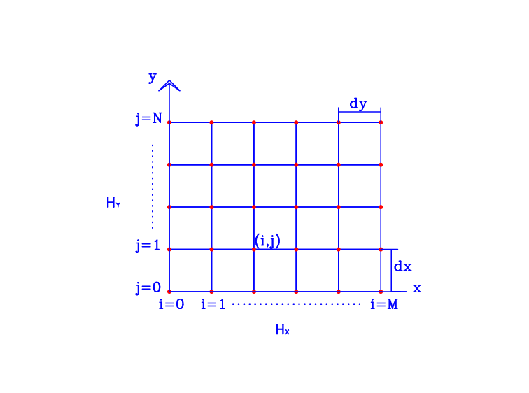
Figure Spatial Grid
Derivatives are replaced by their centered, second-order finite difference approximations
and similarly for the \(y\)-derivatives. The discrete analogue of the (Poisson equation), centered at the point \((x_i,y_j)\), may be written as
or, after rearranging,
(Discrete \(\chi\) Eqn)
Here, we’ve used \(F_{i,j} = F(x_i,y_j,t)\) as the values of the right hand side function at the discrete points, and said nothing of how to discretize \(F\) (this will be left until Right Hand Side. The (Discrete :math:chi` equation <#eq:discrete-chi>`__) is an equation centered at the grid point \((i,j)\), and relating the values of the approximate solution, \(\chi_{i,j}\), at the \((i,j)\) point, to the four neighbouring values, as described by the 5-point difference stencil pictured in Figure Stencil.
[6]:
Image(filename='images/2diff.png',width='40%')
[6]:
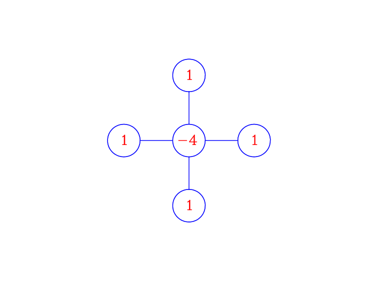
Figure Stencil: The standard 5-point centered difference stencil for the Laplacian (multiply by \(\frac{1}{d^2}\) to get the actual coefficients.
These stencil diagrams are a compact way of representing the information contained in finite difference formulas. To see how useful they are, do the following:
Choose the point on the grid in Figure Spatial Grid that you want to apply the difference formula (Discrete :math:chi` Eqn <#eq:discrete-chi>`__).
Overlay the difference stencil diagram on the grid, placing the center point (with value \(-4\)) on this point.
The numbers in the stencil are the multiples for each of the unknowns \(\chi_{i,j}\) in the difference formula.
An illustration of this is given in Figure Overlay.
[7]:
Image(filename='images/2diffgrid.png',width='40%')
[7]:
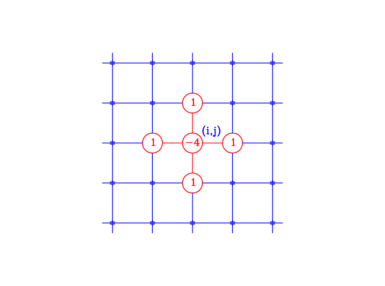
Figure Overlay: The 5-point difference stencil overlaid on the grid.
Before going any further with the discretization, we need to provide a few more details for the discretization of the right hand side function, \(F(x,y,t)\), and the boundary conditions. If you’d rather skip these for now, and move on to the time discretization (Section Temporal Discretization) or the outline of the solution procedure (Section Outline of Solution Procedure), then you may do so now.
Right Hand Side
The right hand side function for the (Poisson equation) is reproduced here in scaled form (with the “primes” dropped):
Alternatively, the Coriolis and Jacobian terms can be grouped together as a single term:
Except for the Jacobian term, straightforward second-order centered differences will suffice for the Coriolis force
the wind stress
and the second order viscosity term
The higher order (biharmonic) viscosity term, \(\nabla_h^4 \psi\), is slightly more complicated. The difference stencil can be derived in a straightforward way by splitting into \(\nabla_h^2 (\nabla_h^2 \psi)\) and applying the discrete version of the Laplacian operator twice. The resulting difference formula is
(Bi-Laplacian)
which is pictured in the difference stencil in Figure Bi-Laplacian Stencil.
[8]:
Image(filename='images/4diff.png',width='40%')
[8]:
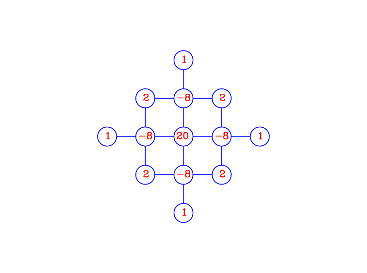
Figure Bi-Laplacian Stencil: 13-point difference stencil for the centered difference formula for \(\nabla_h^4\) (multiply by \(\frac{1}{d^4}\) to get the actual coefficients).
The final term is the Jacobian term, \({\cal J}(\psi, \nabla^2_h\psi)\) which, as you might have already guessed, is the one that is going to give us the most headaches. To get a feeling for why this might be true, go back to (Rescaled Quasi-Geostropic Equation) and notice that the only nonlinearity arises from this term. Typically, it is the nonlinearity in a problem that leads to difficulties in a numerical scheme. Remember the formula given for \({\cal J}\) in the previous section:
(Jacobian: Expansion 1)
Problem One
Apply the standard centered difference formula (see Lab 1 if you need to refresh you memory) to get a difference approximation to the Jacobian based on (Jacobian: Expansion 1. You will use this later in Problem Two.
We’ve seen before that there is usually more than one way to discretize a given expression. This case is no different, and there are many possible ways to derive a discrete version of the Jacobian. Two other approaches are to apply centered differences to the following equivalent forms of the Jacobian:
(Jacobian: Expansion 2)
(Jacobian: Expansion 3)
Each formula leads to a different discrete formula, and we will see in Section Aliasing Error and Nonlinear Instability what effect the non-linear term has on the discrete approximations and how the use of the different formulas affect the behaviour of the numerical scheme. Before moving on, try to do the following two quizzes.
Quiz on Jacobian Expansion #2
Using second order centered differences, what is the discretization of the second form of the Jacobian given by
A:
\[\frac 1 {d^2} \left[ \left( a_{i+1,j} - a_{i-1,j} \right) \left( b_{i,j+1} - b_{i,j-1} \right) - \left( a_{i,j+1} - a_{i,j-1} \right) \left( b_{i+1,j} - b_{i-1,j} \right) \right]\]B:
\[\frac 1 {4d^2} \left[ a_{i+1,j} \left( b_{i+1,j+1} - b_{i+1,j-1} \right) - a_{i-1,j} \left( b_{i-1,j+1} - b_{i-1,j-1} \right) - a_{i,j+1} \left( b_{i+1,j+1} - b_{i-1,j+1} \right) + a_{i,j-1} \left( b_{i+1,j-1} - b_{i-1,j-1} \right) \right]\]C:
\[\frac 1 {d^2} \left[ \left( a_{i+1/2,j} - a_{i-1/2,j} \right) \left( b_{i,j+1/2} - b_{i,j-1/2} \right) - \left( a_{i,j+1/2} - a_{i,j-1/2} \right) \left( b_{i+1/2,j} - b_{i-1/2,j} \right) \right]\]D:
\[\frac 1 {4d^2} \left[ b_{i+1,j} \left( a_{i+1,j+1} - a_{i+1,j-1} \right) - b_{i-1,j} \left( a_{i-1,j+1} - a_{i-1,j-1} \right) - b_{i,j+1} \left( a_{i+1,j+1} - a_{i-1,j+1} \right) + b_{i,j-1} \left( a_{i+1,j-1} - a_{i-1,j-1} \right) \right]\]E:
\[\frac 1 {4d^2} \left[ a_{i+1,j+1} \left( b_{i+1,j+1} - b_{i+1,j-1} \right) - a_{i-1,j-1} \left( b_{i-1,j+1} - b_{i-1,j-1} \right) - a_{i+1,j+1} \left( b_{i+1,j+1} - b_{i-1,j+1} \right) + a_{i-1,j-1} \left( b_{i+1,j-1} - b_{i-1,j-1} \right) \right]\]F:
\[\frac 1 {4d^2} \left[ \left( a_{i+1,j} - a_{i-1,j} \right) \left( b_{i,j+1} - b_{i,j-1} \right) - \left( a_{i,j+1} - a_{i,j-1} \right) \left( b_{i+1,j} - b_{i-1,j} \right) \right]\]G:
\[\frac 1 {4d^2} \left[ b_{i,j+1} \left( a_{i+1,j+1} - a_{i-1,j+1} \right) - b_{i,j-1} \left( a_{i+1,j-1} - a_{i-1,j-1} \right) - b_{i+1,j} \left( a_{i+1,j+1} - a_{i+1,j-1} \right) + b_{i-1,j} \left( a_{i-1,j+1} - a_{i-1,j-1} \right) \right]\]
In the following, replace ‘x’ by ‘A’, ‘B’, ‘C’, ‘D’, ‘E’, ‘F’, ‘G’, or ‘Hint’
[9]:
print (quiz.jacobian_2(answer = 'x'))
Acceptable answers are 'A', 'B', 'C', 'D', 'E', 'F', 'G', 'Hint'
Quiz on Jacobian Expansion #3
Using second order centered differences, what is the discretization of the third form of the Jacobian given by
A: - A:
\[\frac 1 {d^2} \left[ \left( a_{i+1,j} - a_{i-1,j} \right) \left( b_{i,j+1} - b_{i,j-1} \right) - \left( a_{i,j+1} - a_{i,j-1} \right) \left( b_{i+1,j} - b_{i-1,j} \right) \right]\]B:
\[\frac 1 {4d^2} \left[ a_{i+1,j} \left( b_{i+1,j+1} - b_{i+1,j-1} \right) - a_{i-1,j} \left( b_{i-1,j+1} - b_{i-1,j-1} \right) - a_{i,j+1} \left( b_{i+1,j+1} - b_{i-1,j+1} \right) + a_{i,j-1} \left( b_{i+1,j-1} - b_{i-1,j-1} \right) \right]\]C:
\[\frac 1 {d^2} \left[ \left( a_{i+1/2,j} - a_{i-1/2,j} \right) \left( b_{i,j+1/2} - b_{i,j-1/2} \right) - \left( a_{i,j+1/2} - a_{i,j-1/2} \right) \left( b_{i+1/2,j} - b_{i-1/2,j} \right) \right]\]D:
\[\frac 1 {4d^2} \left[ b_{i+1,j} \left( a_{i+1,j+1} - a_{i+1,j-1} \right) - b_{i-1,j} \left( a_{i-1,j+1} - a_{i-1,j-1} \right) - b_{i,j+1} \left( a_{i+1,j+1} - a_{i-1,j+1} \right) + b_{i,j-1} \left( a_{i+1,j-1} - a_{i-1,j-1} \right) \right]\]E:
\[\frac 1 {4d^2} \left[ a_{i+1,j+1} \left( b_{i+1,j+1} - b_{i+1,j-1} \right) - a_{i-1,j-1} \left( b_{i-1,j+1} - b_{i-1,j-1} \right) - a_{i+1,j+1} \left( b_{i+1,j+1} - b_{i-1,j+1} \right) + a_{i-1,j-1} \left( b_{i+1,j-1} - b_{i-1,j-1} \right) \right]\]F:
\[\frac 1 {4d^2} \left[ \left( a_{i+1,j} - a_{i-1,j} \right) \left( b_{i,j+1} - b_{i,j-1} \right) - \left( a_{i,j+1} - a_{i,j-1} \right) \left( b_{i+1,j} - b_{i-1,j} \right) \right]\]G:
\[\frac 1 {4d^2} \left[ b_{i,j+1} \left( a_{i+1,j+1} - a_{i-1,j+1} \right) - b_{i,j-1} \left( a_{i+1,j-1} - a_{i-1,j-1} \right) - b_{i+1,j} \left( a_{i+1,j+1} - a_{i+1,j-1} \right) + b_{i-1,j} \left( a_{i-1,j+1} - a_{i-1,j-1} \right) \right]\]
In the following, replace ‘x’ by ‘A’, ‘B’, ‘C’, ‘D’, ‘E’, ‘F’, ‘G’, or ‘Hint’
[10]:
print (quiz.jacobian_3(answer = 'x'))
Acceptable answers are 'A', 'B', 'C', 'D', 'E', 'F', 'G', 'Hint'
Boundary Conditions
One question that arises immediately when applying the difference stencils in Figure Stencil and Figure Bi-Laplacian Stencil is
What do we do at the boundary, where at least one of the nodes of the difference stencil lies outside of the domain?
The answer to this question lies with the boundary conditions for \(\chi\) and \(\psi\). We already know the boundary conditions for \(\psi\) from Section The Quasi-Geostrophic Model:
Free slip:
The free slip boundary condition, \(\psi=0\), is applied when \(A_h=0\), which we can differentiate with respect to time to get the identical condition \(\chi=0\). In terms of the discrete unknowns, this translates to the requirement that
\[\Psi_{0,j} = \Psi_{N,j} = \Psi_{i,0} = \Psi_{i,N} = 0 \;\; \mbox{ for} \; i,j = 0,1,\ldots,N,\]
and similarly for \(\chi\). All boundary values for \(\chi\) and \(\Psi\) are known, and so we need only apply the difference stencils at interior points (see Figure Ghost Points). When \(A_h=0\), the high-order viscosity term is not present, and so the only stencil appearing in the discretization is the 5-point formula (the significance of this will become clear when we look at no-slip boundary conditions).
[11]:
Image(filename='images/ghost3.png',width='50%')
[11]:
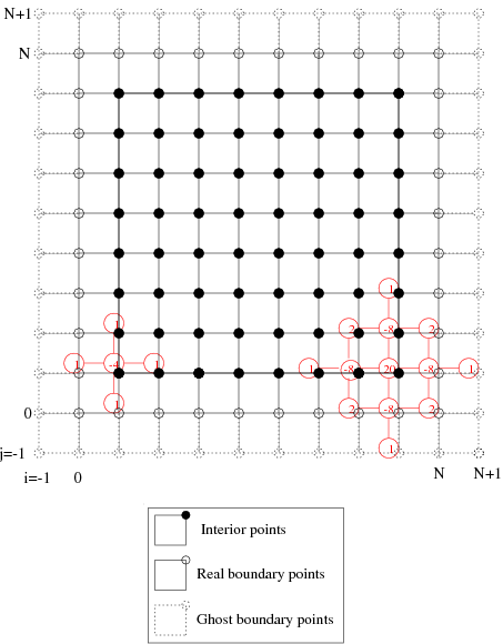
Figure Ghost Points: The points on the computational grid, which are classified into interior, real boundary, and ghost boundary points. The 5- and 13-point difference stencils, when overlaid on the grid, demonstrate that only the real boundary values are needed for the free-slip boundary values (when \(A_h=0\)), while ghost points must be introduced for the no-slip conditions (when \(A_h\neq 0\), and the higher order viscosity term is present).
No-slip:
The no-slip conditions appear when \(A_h\neq 0\), and include the free slip conditions \(\psi=\chi=0\) (which we already discussed above), and the normal derivative condition \(\nabla\psi\cdot\hat{n}=0\), which must be satisfied at all boundary points. It is clear that if we apply the standard, second-order centered difference approximation to the first derivative, then the difference stencil extends beyond the boundary of the domain and contains at least one non-existent point! How can we get around this problem?
The most straightforward approach (and the one we will use in this Lab) is to introduce a set of fictitious points or ghost points,
\[\Psi_{-1,j}, \;\; \Psi_{N+1,j}, \;\; \Psi_{i,-1}, \;\; \Psi_{i,N+1}\]
for \(i,j=0,1,2,\ldots,N+1\), which extend one grid space outside of the domain, as shown in Figure Ghost Points. We can then discretize the Neumann condition in a straightforward manner. For example, consider the point \((0,1)\), pictured in Figure No Slip Boundary Condition, at which the discrete version of \(\nabla\psi\cdot\hat{n}=0\) is
\[\frac{1}{2d} ( \Psi_{1,1} - \Psi_{-1,1}, \Psi_{0,2} - \Psi_{0,0} ) \cdot (-1,0) = 0,\]
(where \((-1,0)\) is the unit outward normal vector), which simplifies to
\[\Psi_{-1,1} = \Psi_{1,1}.\]
The same can be done for all the remaining ghost points: the value of \(\Psi\) at at point outside the boundary is given quite simply as the value at the corresponding interior point reflected across the boundary.
[12]:
Image(filename='images/noslip.png',width='40%')
[12]:
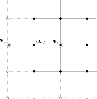
Figure No Slip Boundary Condition: The discrete Neumann boundary conditions are discretized using ghost points. Here, at point \((0,1)\), the unit outward normal vector is \(\hat{n}=(-1,0)\), and the discrete points involved are the four points circled in red. The no-slip condition simply states that \(\Psi_{-1,1}\) is equal to the interior value \(\Psi_{1,1}\).
Now, remember that when \(A_h\neq 0\), the \(\nabla_h^4\psi\) term appears in the equations, which is discretized as a 13-point stencil . Looking at Figure Ghost Points, it is easy to see that when the 13-point stencil is applied at points adjacent to the boundary (such as \((N-1,N-1)\) in the Figure) it involves not only real boundary points, but also ghost boundary points (compare this to the 5-point stencil). But, as we just discovered above, the presence of the ghost points in the stencil poses no difficulty, since these values are known in terms of interior values of \(\Psi\) using the boundary conditions.
Just as there are many Runge-Kutta schemes, there are many finite difference stencils for the different derivatives. For example, one could use a 5-point, \(\times\)-shaped stencil for \(\nabla^2\psi\). The flexibility of having several second-order stencils is what makes it possible to determine an energy- and enstrophy-conserving scheme for the Jacobian which we do later.
A good discussion of boundary conditions is given by McCalpin in his QGBOX code documentation, on page 44.
Matrix Form of the Discrete Equations
In order to write the discrete equations in matrix form, we must first write the unknown values \(\chi_{i,j}\) in vector form. The most obvious way to do this is to traverse the grid (see Figure Spatial Grid), one row at a time, from left to right, leaving out the known, zero boundary values, to obtain the ordering:
and similarly for \(\vec{F}\). The resulting matrix (with this ordering of unknowns) results in a matrix of the form given in Figure Matrix.
[13]:
Image(filename='images/matrix.png',width='40%')
[13]:
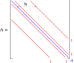
Figure Matrix: The matrix form for the discrete Laplacian. The 5 diagonals (displayed in blue and red) represent the non-zero values in the matrix \(-\) all other values are zero.
The diagonals with the 1’s (pictured in red) contain some zero entries due to the boundary condition \(u=0\). Notice how similar this matrix appears to the tridiagonal matrix in the Problems from Lab 3, which arose in the discretization of the second derivative in a boundary value problem. The only difference here is that the Laplacian has an additional second derivative with respect to \(y\), which is what adds the additional diagonal entries in the matrix.
Before you think about running off and using Gaussian elimination (which was reviewed in Lab 3), think about the size of the matrix you would have to solve. If \(N\) is the number of grid points, then the matrix is size \(N^2\)-by-\(N^2\). Consequently, Gaussian elimination will require on the order of \(N^6\) operations to solve the matrix only once. Even for moderate values of \(N\), this cost can be prohibitively expensive. For example, taking \(N=101\) results in a \(10000\times 10000\) system of linear equations, for which Gaussian elimination will require on the order of \(10000^3=10^{12}\) operations! As mentioned in Lab 3, direct methods are not appropriate for large sparse systems such as this one. A more appropriate choice is an iterative or relaxation scheme, which is the subject of the next section..
Solution of the Poisson Equation by Relaxation
One thing to notice about the matrix in Figure Matrix is that it contains many zeros. Direct methods, such as Gaussian elimination (GE), are so inefficient for this problem because they operate on all of these zero entries (in fact, there are other direct methods that exploit the sparse nature of the matrix to reduce the operation count, but none are as efficient as the methods we will talk about here).
However, there is another class of solution methods, called iterative methods (refer to Lab 3) which are natural candidates for solving such sparse problems. They can be motivated by the fact that since the discrete equations are only approximations of the PDE to begin with, why should we bother computing an exact solution to an approximate problem? Iterative methods are based on the notion that one sets up an iterative procedure to compute successive approximations to the solution \(-\) approximations that get closer and closer to the exact solution as the iteration proceeds, but never actually reach the exact solution. As long as the iteration converges and the approximate solution gets to within some tolerance of the exact solution, then we are happy! The cost of a single iterative step is designed to depend on only the number of non-zero elements in the matrix, and so is considerably cheaper than a GE step. Hence, as long as the iteration converges in a “reasonable number” of steps, then the iterative scheme will outperform GE.
Iterative methods are also know as relaxation methods, of which the Jacobi method is the simplest. Here are the basic steps in the Jacobi iteration (where we’ve dropped the time superscript \(p\) to simplify the notation):
Take an initial guess, \(\chi_{i,j}^{(0)}\). Let \(n=0\).
For each grid point \((i,j)\), compute the residual vector
\[R_{i,j}^{(n)} = F_{i,j} - \nabla^2\chi^{(n)}_{i,j}\]\[= F_{i,j} - \frac{1}{d^2} ( \chi_{i+1,j}^{(n)} + \chi_{i,j+1}^{(n)} + \chi_{i-1,j}^{(n)} +\chi_{i,j-1}^{(n)} - 4 \chi_{i,j}^{(n)} )\](which is non-zero unless \(\chi_{i,j}\) is the exact solution).
You should not confuse the relaxation iteration index (superscript \(\,^{(n)}\)) with the time index (superscript \(\,^p\)). Since the relaxation iteration is being performed at a single time step, we’ve dropped the time superscript for now to simplify notation. Just remember that all of the discrete values in the relaxation are evaluated at the current time level \(p\).
“Adjust” \(\chi_{i,j}^{(n)}\), (leaving the other neighbours unchanged) so that \(R_{i,j}^{(n)}=0\). That is, replace \(\chi_{i,j}^{(n)}\) by whatever you need to get a zero residual. This replacement turns out to be:
\[\chi_{i,j}^{(n+1)} = \chi_{i,j}^{(n)} - \frac{d^2}{4} R_{i,j}^{(n)},\]which defines the iteration.
Set \(n\leftarrow n+1\), and repeat steps 2 & 3 until the residual is less than some tolerance value. In order to measure the size of the residual, we use a relative maximum norm measure, which says
\[d^2 \frac{\|R_{i,j}^{(n)}\|_\infty}{\|\chi_{i,j}^{(n)}\|_\infty} < TOL\]where
\[\|R_{i,j}^{(n)}\|_\infty = \max_{i,j} |R_{i,j}^{(n)}|\]is the max-norm of \(R_{i,j}\), or the maximum value of the residual on the grid (there are other error tolerances we could use but this is one of the simplest and most effective). Using this measure for the error ensures that the residual remains small relative to the solution, \(\chi_{i,j}\). A typical value of the tolerance that might be used is \(TOL=10^{-4}\).
There are a few important things to note about the basic relaxation procedure outlined above
This Jacobi method is the simplest form of relaxation. It requires that you have two storage vectors, one for \(\chi_{i,j}^{(n)}\) and one for \(\chi_{i,j}^{(n+1)}\).
The relaxation can be modified by using a single vector to store the \(\chi\) values. In this case, as you compute the residual vector and update \(\chi\) at each point \((i,j)\), the residual involves some \(\chi\) values from the previous iteration and some that have already been updated. For example, if we traverse the grid by rows (that is, loop over \(j\) first and then \(i\)), then the residual is now given by
\[R_{i,j}^{(n)} = F_{i,j} - \frac{1}{d^2} ( \chi_{i+1,j}^{(n)} + \chi_{i,j+1}^{(n)} + \underbrace{\chi_{i-1,j}^{(n+1)} + \chi_{i,j-1}^{(n+1)}}_{\mbox{{updated already}}} - 4 \chi_{i,j}^{(n)} ),\](where the \((i,j-1)\) and \((i-1,j)\) points have already been updated), and then the solution is updated
\[\chi_{i,j}^{(n+1)} = \chi_{i,j}^{(n)} - \frac{d^2}{4} R_{i,j}^{(n)}.\]Not only does this relaxation scheme save on storage (since only one solution vector is now required), but it also converges more rapidly (typically, it takes half the number of iterations as Jacobi), which speeds up convergence somewhat, but still leaves the cost at the same order as Jacobi, as we can see from Cost of Schemes Table. This is known as the Gauss-Seidel relaxation scheme.
In practice, we actually use a modification of Gauss-Seidel
\[\chi_{i,j}^{(n+1)} = \chi_{i,j}^{(n)} - \frac{\mu d^2}{4} R_{i,j}^{(n)}\]where \(1<\mu<2\) is the relaxation parameter. The resulting scheme is called successive over-relaxation, or SOR, and it improves convergence considerably (see Cost of Schemes Table.
What happens when \(0<\mu<1\)? Or \(\mu>2\)? The first case is called under-relaxation, and is useful for smoothing the solution in multigrid methods. The second leads to an iteration that never converges.
Does the iteration converge? For the Poisson problem, yes, but not in general.
How fast does the iteration converge? and How much does each iteration cost? The answer to both of these questions gives us an idea of the cost of the relaxation procedure …
Assume we have a grid of size \(N\times N\). If we used Gaussian elimination to solve this matrix system (with \(N^2\) unknowns), we would need to perform on the order of \(N^6\) operations (you saw this in Lab #3). One can read in any numerical linear algebra textbook (Strang 1988, for example), that the number of iterations required for Gauss-Seidel and Jacobi is on the order of \(N^3\), while for SOR it reduces to \(N^2\). There is another class of iterative methods, called multigrid methods, which converge in a constant number of iterations (the optimal result)
If you look at the arithmetic operations performed in the the relaxation schemes described above, it is clear that a single iteration involves on the order of \(N^2\) operations (a constant number of multiplications for each point).
Putting this information together, the cost of each iterative scheme can be compared as in Cost of Schemes Table.
Method |
Order of Cost |
|---|---|
Gaussian Elimination |
\(N^6\) |
Jacobi |
\(N^5\) |
Gauss-Seidel |
\(N^5\) |
SOR |
\(N^4\) |
Multigrid |
\(N^2\) |
Cost of Schemes Table: Cost of iterative schemes compared to direct methods.
Multigrid methods are obviously the best, but are also extremely complicated … we will stick to the much more manageable Jacobi, Gauss-Seidel and SOR schemes.
There are other methods (called conjugate gradient and capacitance matrix methods) which improve on the relaxation methods we’ve seen. These won’t be described here.
Temporal Discretization
Let us now turn to the time evolution equation for the stream function. Supposing that the initial time is \(t=0\), then we can approximate the solution at the discrete time points \(t_p = p\Delta t\), and write the discrete solution as
Notice that the spatial indices appear as subscripts and the time index as a superscript on the discrete approximation \(\chi\).
We can choose any discretization for time that we like, but for the QG equation, it is customary (see Mesinger and Arakawa, for example) to use a centered time difference to approximate the derivative in :
or, after rearranging,
(Leapfrog Eqn)
This time differencing method is called the leap frog scheme, and was introduced in Lab 7. A pictorial representation of this scheme is given in Figure Leap-Frog Scheme.
[14]:
Image(filename='images/leapfrog.png',width='40%')
[14]:
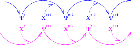
Figure Leap-Frog Scheme: A pictorial representation of the “leap-frog” character of the time-stepping scheme. The values of \(\chi\) at even time steps are linked together with the odd \(\Psi\) values; likewise, values of \(\chi\) at odd time steps are linked to the even \(\Psi\) values.
There are two additional considerations related to the time discretization:
The viscous terms (\(\nabla_h^2\psi\) and \(\nabla_h^4\psi\)) are evaluated at the \(p-1\) time points, while all other terms in the right hand side are evaluated at \(p\) points. The reasoning for this is described in McCalpin’s QGBOX documentation [p. 8]:
Note that the frictional terms are all calculated at the old \((n-1)\) time level, and are therefore first-order accurate in time. This ’time lagging’ is necessary for linear computational stability.
This second item will not be implemented in this lab or the problems, but should still be kept in mind …
The leap-frog time-stepping scheme has a disadvantage in that it introduces a “computational mode” … McCalpin [p. 23] describes this as follows:
Leap-frog models are plagued by a phenomenon called the “computational mode”, in which the odd and even time levels become independent. Although a variety of sophisticated techniques have been developed for dealing with this problem, McCalpin’s model takes a very simplistic approach. Every narg* time steps, adjacent time levels are simply averaged together (where narg\(\approx 100\) and odd)*
Why don’t we just abandon the leap-frog scheme? Well, Mesinger and Arakawa [p. 18] make the following observations regarding the leap-frog scheme:
its advantages: simple and second order accurate; neutral within the stability range.
its disadvantages: for non-linear equations, there is a tendency for slow amplification of the computational mode.
the usual method for suppressing the spurious mode is to insert a step from a two-level scheme occasionally (or, as McCalpin suggests, to occasionally average the solutions at successive time steps).
In Chapter 4, they mention that it is possible to construct grids and/or schemes with the same properties as leap-frog and yet the computational mode is absent.
The important thing to get from this is that when integrating for long times, the computational mode will grow to the point where it will pollute the solution, unless one of the above methods is implemented. For simplicity, we will not be worrying about this in Lab #8.
Outline of Solution Procedure
Now that we have discretized in both space and time, it is possible to outline the basic solution procedure.
Assume that at \(t=t_p\), we know \(\Psi^0, \Psi^1, \dots, \Psi^{p-1}\)
Calculate \(F_{i,j}^p\) for each grid point \((i,j)\) (see Section Right Hand Side). Keep in mind that the viscosity terms (\(\nabla_h^2\psi\) and \(\nabla_h^4\psi\)) are evaluated at time level \(p-1\), while all other terms are evaluated at time level \(p\) (this was discussed in Section Temporal Discretization).
Solve the (Discrete :math:chi` equation <#eq:discrete-chi>`__) for \(\chi_{i,j}^p\) (the actual solution method will be described in Section Solution of the Poisson Equation by Relaxation.
Given \(\chi_{i,j}^p\), we can find \(\Psi_{i,j}^{p+1}\) by using the (Leap-frog time stepping scheme)
Let \(p \leftarrow p+1\) and return to step 2.
Notice that step 1 requires a knowledge of two starting values, \(\Psi^0\) and \(\Psi^1\), at the initial time. An important addition to the procedure below is some way to get two starting values for \(\Psi\). Here are several alternatives:
Set \(\Psi^0\) and \(\Psi^1\) both to zero.
Set \(\Psi^0=0\), and then use a forward Euler step to find \(\Psi^1\).
Use a predictor-corrector step, like that employed in Lab 7.
Problem Two
Now that you’ve seen how the basic numerical scheme works, it’s time to jump into the numerical scheme. The code has already been written for the discretization described above, with free-slip boundary conditions and the SOR relaxation scheme. The code is in qg.py and the various functions are:
- main
the main routine, contains the time-stepping and the output.
- param()
sets the physical parameters of the system.
- numer_init()
sets the numerical parameters.
- vis(psi, nx, ny)
calculates the second order (\(\nabla^2\)) viscosity term (not leap-frogged).
- wind(psi, nx, ny)
calculates the the wind term.
- mybeta(psi, nx, ny)
calculates the beta term
- jac(psi, vis, nx, ny)
calculate the Jacobian term. (Arakawa Jacobian given here).
- chi(psi, vis_curr, vis_prev, chi_prev, nx, ny, dx, r_coeff, tol, max_count, epsilon, wind_par, vis_par)
calculates \(\chi\) using a call to relax
- relax(rhs, chi_prev, dx, nx, ny, r_coeff, tol, max_count)
does the relaxation.
Your task in this problem is to program the “straightforward” discretization of the Jacobian term, using (Jacobian: Expansion 1), that you derived in Problem One. The only change this involves is inserting the code into the function jac. Once finished, run the code. The parameter functions param init_numer provide some sample parameter values for you to execute the code with. Try these input values and observe what happens in the solution. Choose one of the physical parameters to vary. Does changing the parameter have any effect on the solution? in what way?
Hand in the code for the Jacobian, and a couple of plots demonstrating the solution as a function of parameter variation. Describe your results and make sure to provide parameter values to accompany your explanations and plots.
If the solution is unstable, check your CFL condition. The relevant waves are Rossby waves with wave speed:
\[c=\beta k^{-2}\]where \(k\) is the wave-number. The maximum wave speed is for the longest wave, \(k=\pi/b\) where \(b\) is the size fo your domain.
If the code is still unstable, even though the CFL is satisfied, see Section Aliasing Error and Nonlinear Instability. The solution is nonlinear unstable. Switch to the Arakawa Jacobian for stability.
Problem Three
The code provided for Problem Two implements the SOR relaxation scheme. Your job in this problem is to modify the relaxation code to perform a Jacobi iteration.
Hand in a comparison of the two methods, in tabular form. Use two different relaxation parameters for the SOR scheme. (Include a list of the physical and numerical parameter you are using). Also submit your code for the Jacobi relaxation scheme.
Problem Four
Modify the code to implement the no-slip boundary conditions.
Problem Five
The code you’ve been working with so far uses the simplest possible type of starting values for the unknown stream function: both are set to zero. If you’re keen to play around with the code, you might want to try modifying the SOR code for the two other methods of computing starting values: using a forward Euler step, or a predictor-corrector step (see Section Outline of Solution Procedure).
Aliasing Error and Nonlinear Instability
In Problem Two, you encountered an example of the instability that can occur when computing numerical solutions to some nonlinear problems, of which the QG equations is just one example. This effect has in fact been known for quite some time. Early numerical experiments by N. Phillips in 1956 exploded after approximately 30 days of integration due to nonlinear instability. He used the straightforward centered difference formula for as you did.
It is important to realize that this instability does not occur in the physical system modeled by the equations of motion. Rather is an artifact of the discretization process, something known as aliasing error. Aliasing error can be best understood by thinking in terms of decomposing the solution into modes. In brief, aliasing error arises in non-linear problems when a numerical scheme amplifies the high-wavenumber modes in the solution, which corresponds physically to a spurious addition of energy into the system. Regardless of how much the grid spacing is reduced, the resulting computation will be corrupted, since a significant amount of energy is present in the smallest resolvable scales of motion. This doesn’t happen for every non-linear problem or every difference scheme, but is an issue that one who is using numerical codes must be aware of.
Example One
Before moving on to how we can handle the instability in our discretization of the QG equations, you should try out the following demo on aliasing error. It is taken from an example in Mesinger and Arakawa [p. 35ff.], based on the simplest of non-linear PDE’s, the advection equation:
\[\frac{du}{dt}+u\frac{du}{dx} = 0.\]If we decompose the solution into Fourier mode, and consider a single mode with wavenumber \(k\),
\[u(x) = \sin{kx}\]then the solution will contain additional modes, due to the non-linear term, and given by
\[u \frac{du}{dx} = k \sin{kx} \cos{kx} =\frac{1}{2}k \sin{2kx}.\]
With this as an introduction, keep the following in mind while going through the demo:
on a computational grid with spacing \(\Delta x\), the discrete versions of the modes can only be resolved up to a maximum wavenumber, \(k_{max}=\frac{\pi}{\Delta x}\).
even if we start with modes that are resolvable on the grid, the non-linear term introduces modes with a higher wavenumber, which may it not be possible to resolve. These modes, when evaluated at discrete points, appear as modes with lower wavenumber; that is, they are aliased to the lower modes (this becomes evident in the demo as the wavenumber is increased …).
not only does aliasing occur, but for this problem, these additional modes are amplified by a factor of \(\frac{1}{2}k\). This is the source of the aliasing error – such amplified modes will grow in time, no matter how small the time step taken, and will pollute the computations.
The previous example is obviously a much simpler non-linearity than that of the QG equations, but the net effect is the same. The obvious question we might ask now is:
Can this problem be averted for our discretization of the QG equations with the leap-frog time-stepping scheme, or do we have to abandon it?
There are several possible solutions, presented by Mesinger and Arakawa [p. 37], summarized here, including
filter out the top half or third of the wavenumbers, so that the aliasing is eliminated.
use a differencing scheme that has a built-in damping of the shortest wavelengths.
the most elegant, and one that allows us to continue using the leap-frog time stepping scheme, is one suggested by Arakawa, is one that aims to eliminate the spurious inflow of energy into the system by developing a discretization of the Jacobian term that satisfies discrete analogues of the conservation properties for average vorticity, enstrophy and kinetic energy.
This third approach will be the one we take here. The details can be found in the Mesinger-Arakawa paper, and are not essential here; the important point is that there is a discretization of the Jacobian that avoids the instability problem arising from aliasing error. This discrete Jacobian is called the Arakawa Jacobian and is obtained by averaging the discrete Jacobians obtained by using standard centered differences on the formulae (Jacobian: Expansion 1), (Jacobian: Expansion 2) and (Jacobian: Expansion 3) (see Problem One and the two quizzes following it in Section Right Hand Side.
You will not be required to derive or code the Arakawa Jacobian (the details are messy!), and the code will be provided for you for all the problems following Problem Two.
Classical Solutions
Bryan (1963) and Veronis (1966)
Problem Six
Mathematical Notes
Definition of the Beta-plane
A \(\beta\)-plane is a plane approximation of a curved section of the Earth’s surface, where the Coriolis parameter, \(f(y)\), can be written roughly as a linear function of \(y\)
for \(f_0\) and \(\beta\) some constants. The motivation behind this approximation follows.
[15]:
Image(filename='images/coriolis.png',width='30%')
[15]:
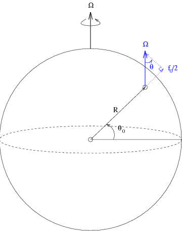
Figure Rotating Globe: A depiction of the earth and its angular frequency of rotation, \(\Omega\), the local planetary vorticity vector in blue, and the Coriolis parameter, \(f_0\), at a latitude of \(\theta_0\).
Consider a globe (the earth) which is rotating with angular frequency \(\Omega\) (see Figure Rotating Globe), and assume that the patch of ocean under consideration is at latitude \(\theta\). The most important component of the Coriolis force is the local vertical (see the in Figure Rotating Globe), which is defined in terms of the Coriolis parameter, \(f\), to be
This expression may be simplified somewhat by ignoring curvature effects and approximating the earth’s surface at this point by a plane \(-\) if the plane is located near the middle latitudes, then this is a good approximation. If \(\theta_0\) is the latitude at the center point of the plane, and \(R\) is the radius of the earth (see Figure Rotating Globe), then we can apply trigonometric ratios to obtain the following expression on the plane:
Not surprisingly, this plane is called a mid-latitude :math:`beta`-plane.
[16]:
Image(filename='images/beta-plane.png',width='30%')
[16]:
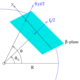
Figure Beta-plane: The \(\beta\)-plane approximation, with points on the plane located along the local \(y\)-axis. The Coriolis parameter, \(f\), at any latitude \(\theta\), can be written in terms of \(y\) using trigonometric ratios.
Simplification of the QG Model Equations
The first approximation we will make eliminates several of the non-linear terms in the set of equations: (X-Momentum Eqn), (Y-Momentum Eqn), (Hydrostatic Eqn) and (Continuity Eqn). A common simplification that is made in this type of flow is the quasi-geostrophic (QG) approximation, where the horizontal pressure gradient and horizontal components of the Coriolis force are matched:
Remembering that the fluid is homogeneous (the density is constant), (Continuity Eqn) implies
We can then differentiate the QG balance equations to obtain
Therefore, the terms \(w \, \partial u/\partial z\) and \(w \, \partial v/\partial z\) can be neglected in ((X-Momentum Eqn)) and ((Y-Momentum Eqn)).
The next simplification is to eliminate the pressure terms in ((X-Momentum Eqn)) and ((Y-Momentum Eqn)) by cross-differentiating. If we define the vorticity
then we can cross-differentiate the two momentum equations and replace them with a single equation in \(\zeta\):
where \(\beta \equiv df/dy\). Notice the change in notation for derivatives, from \(\nabla\) to \(\nabla_h\): this indicates that derivative now appear only with respect to the “horizontal” coordinates, \(x\) and \(y\), since the \(z\)-dependence in the solution has been eliminated.
The third approximation we will make is to assume that vorticity effects are dominated by the Coriolis force, or that \(|\zeta| \ll f\). Using this, along with the (Continuity Eqn) implies that
(Vorticity Eqn)
The reason for making this simplification may not be obvious now but it is a good approximation in flows in the ocean and, as we will see next, it allows us to eliminate the Coriolis term.
The final sequence of simplifications eliminate the \(z\)-dependence in the problem by integrating (Vorticity Eqn) in the vertical direction and using boundary conditions.
The top 500 metres of the ocean tend to act as a single slab-like layer. The effect of stratification and rotation cause mainly horizontal motion. To first order, the upper layers are approximately averaged flow (while to the next order, surface and deep water move in opposition with deep flow much weaker). Consequently, our averaging over depth takes into account this “first order” approximation embodying the horizontal (planar) motion, and ignoring the weaker (higher order) effects.
First, recognize that the vertical component of velocity on both the top and bottom surfaces should be zero:
Notice that the in second condition we’ve also assumed that the water surface is approximately flat \(-\) this is commonly known as the rigid lid approximation. Integrate the differential equation (Vorticity Eqn) with respect to \(z\), applying the above boundary conditions, and using the fact that \(u\) and \(v\) (and therefore also \(\zeta\)) are independent of \(z\),
(Depth-Integrated Vorticity)
The two boundary terms on the right hand side can be rewritten in terms of known information if we apply two additional boundary conditions: the first, that the given wind stress on the ocean surface,
can be written as
which, after differentiating, leads to
(Stress Boundary Condition)
and, the second, that the Ekman layer along the bottom of the ocean, \(z=-H\), generates Ekman pumping which obeys the following relationship:
(Ekman Boundary Condition)
where the Ekman number, \(\kappa\), is defined by
Using (Stress Boundary Condition) and (Ekman Boundary Condition) to replace the boundary terms in (Depth-Integrated Vorticity), we get the following equation for the vorticity:
The next and final step may not seem at first to be much of a simplification, but it is essential in order to derive a differential equation that can be easily solved numerically. Integrate (Continuity Eqn) with respect to \(z\) in order to obtain
after which we can introduce a stream function, \(\psi\), defined in terms of the velocity as
The stream function satisfies this equation exactly, and we can write the vorticity as
which then allows us to write both the velocity and vorticity in terms of a single variable, \(\psi\).
After substituting into the vorticity equation, we are left with a single equation in the unknown stream function.
where
is called the Jacobian operator.
The original system (X-Momentum Eqn), (Y-Momentum Eqn), (Hydrostatic Eqn) and (Continuity Eqn) was a system of four non-linear PDE’s, in four independent variables (the three velocities and the pressure), each of which depend on the three spatial coordinates. Now let us review the approximations made above, and their effects on this system:
After applying the QG approximation and homogeneity, two of the non-linear terms were eliminated from the momentum equations, so that the vertical velocity, \(w\), no longer appears.
By introducing the vorticity, \(\zeta\), the pressure was eliminated, and the two momentum equations to be rewritten as a single equation in \(\zeta\) and the velocities.
Some additional terms were eliminated by assuming that Coriolis effects dominate vorticity, and applying the continuity condition.
Integrating over the vertical extent of the ocean, and applying boundary conditions eliminated the \(z\)-dependence in the problem.
The final step consists of writing the unknown vorticity and velocities in terms of the single unknown stream function, \(\psi\).
It is evident that the final equation is considerably simpler: it is a single, non-linear PDE for the unknown stream function, \(\psi\), which is a function of only two independent variables. As we will see in the next section, this equation is of a very common type, for which simple and efficient numerical techniques are available.
Glossary
advection: A property or quantity transferred by the flow of a fluid is said to be “advected” by the flow. aliasing error: In a numerical scheme, this is the phenomenon that occurs when a grid is not fine enough to resolve the high modes in a solution. These high waveumbers consequently appear as lower modes in the solution due to aliasing. If the scheme is such that these high wavenumber modes are amplified, then the aliased modes can lead to a significant error in the computed solution.
:math:`beta`-plane: A \(\beta\)-plane is a plane approximation of a curved section of the Earth’s surface, where the Coriolis parameter can be written roughly as a linear function.
continuity equation: The equation that describes mass conservation in a fluid, \({\partial \rho}/{\partial t} + \nabla \cdot (\rho \vec u) = 0\)
Coriolis force: An additional force experienced by an observer positioned in a rotating frame of reference. If \(\Omega\) is the angular velocity of the rotating frame, and \(\vec u\) is the velocity of an object observed within the rotating frame, then the Coriolis force, \(\Omega \times \vec u\), appears as a force tending to deflect the moving object to the right.
Coriolis parameter: The component of the planetary vorticity which is normal to the earth’s surface, usually denoted by f.
difference stencil: A convenient notation for representing difference approximation formula for derivatives.
Ekman layer: The frictional layer in a geophysical fluid flow field which appears on a rigid surface perpendicular to the rotation vector.
Gauss-Seidel relaxation: One of a class of iterative schemes for solving systems of linear equations. See Lab 8 for a complete discussion.
homogeneous fluid: A fluid with constant density. Even though the density of ocean water varies with depth, it is often assumed homogeneous in order to simplify the equations of motion.
hydrostatic balance: A balance, in the vertical direction, between the vertical pressure gradient and the buoyancy force. The pressure difference between any two points on a vertical line is assumed to depend only on the weight of the fluid between the points, as if the fluid were at rest, even though it is actually in motion. This approximation leads to a simplification in the equations of fluid flow, by replacing the vertical momentum equation.
incompressible fluid: A fluid for which changes in the density with pressure are negligible. For a fluid with velocity field, \(\vec u\), this is expressed by the equation \(\nabla \cdot \vec u = 0\). This equation states that the local increase of density with time must be balanced by the divergence of the mass flux.
Jacobi relaxation: The simplest of the iterative methods for solving linear systems of equations. See Lab 8 for a complete discussion.
momentum equation(s): The equations representing Newton’s second law of motion for a fluid. There is one momentum equation for each component of the velocity.
over-relaxation: Within a relaxation scheme, this refers to the use of a relaxation parameter \(\mu > 1\). It accelerates the standard Gauss-Seidel relaxation by forcing the iterates to move closer to the actual solution.
Poisson equation: The partial differential equation \(\nabla^2 u = f\) or, written two dimensions, \({\partial^2 u}/{\partial x^2} + {\partial^2 u}/{\partial y^2} =f(x,y)\).
QG: abbreviation for quasi-geostrophic.
quasi-geostrophic balance: Approximate balance between the pressure gradient and the Coriolis Force.
relaxation: A term that applies to a class of iterative schemes for solving large systems of equations. The advantage to these schemes for sparse matrices (compared to direct schemes such as Gaussian elimination) is that they operate only on the non-zero entries of the matrix. For a description of relaxation methods, see Lab 8.
rigid lid approximation: Assumption that the water surface deflection is negligible in the continuity equation (or conservation of volume equation)
SOR: see successive over-relaxation.
sparse system: A system of linear equations whose matrix representation has a large percentage of its entries equal to zero.
stream function: Incompressible, two-dimensional flows with velocity field \((u,v)\), may be described by a stream function, \(\psi(x, y)\), which satisfies \(u = −{\partial \psi}/{\partial y}, v = {\partial \psi}/{\partial x}\). These equations are a consequence of the incompressibility condition.
successive over-relaxation: An iterative method for solving large systems of linear equations. See Lab 8 for a complete discussion.
under-relaxation: Within a relaxation scheme, this refers to the use of a relaxation parameter \(\mu < 1\). It is not appropriate for solving systems of equations directly, but does have some application to multigrid methods.
vorticity: Defined to be the curl of the velocity field, \(\zeta = \nabla \times \vec u\). In geophysical flows, where the Earth is a rotating frame of reference, the vorticity can be considered as the sum of a relative vorticity (the curl of the velocity in the nonrotating frame) and the planetary vorticity, \(2 \Omega\). For these large-scale flows, vorticity is almost always present, and the planetary vorticity dominates.
References
Arakawa, A. and V. R. Lamb, 1981: A potential enstrophy and energy conserving scheme for the shallow water equations. Monthly Weather Review, 109, 18–36.
Bryan, K., 1963: A numerical investigation of a non-linear model of a wind-driven ocean. Journal of Atmospheric Science, 20, 594–606
On the adjustment of azimuthally perturbed vortices. Journal of Geophysical Research, 92, 8213–8225.
Mesinger, F. and A. Arakawa, 1976: Numerical Methods Used in Atmospheric Models,GARP Publications Series No.~17, Global Atmospheric Research Programme.
Pedlosky, J., 1987: Geophysical Fluid Dynamics. Springer-Verlag, New York, 2nd edition.Pond,
Phillips, N. A., 1956: The general circulation of the atmosphere: A numerical experiment. Quarterly Journal of the Royal Meteorological Society, 82, 123–164.
Strang, G., 1988: Linear Algebra and its Applications. Harcourt Brace Jovanovich, San Diego, CA, 2nd edition.
Veronis, G., 1966: Wind-driven ocean circulation – Part 2. Numerical solutions of the non- linear problem. Deep Sea Research, 13, 31–55.
[ ]: