Laboratory 1: An Introduction to the Numerical Solution of Differential Equations: Discretization (2020/Jan/6)
John M. Stockie
List of Problems
Objectives
The examples and exercises in this lab are meant to illustrate the limitations of analytical solution techniques, using several differential equation models for simple physical systems. This is the prime motivation for the use of numerical methods.
After completing this lab, you will understand the process of discretizing a continuous problem, and be able to derive a simple finite difference approximation for an ordinary or partial differential equation. The examples will also introduce the concepts of accuracy and stability, which will be discussed further in Lab 2.
Specifically you will be able to:
Define the term or identify: Ordinary Differential Equation, Partial Differential Equation, Linear equation, Non-linear equation, Initial value problem, Boundary value problem, Open Domain, and Closed Domain.
Define the term, identify or perform: Forward difference discretization, Backward difference discretization, and Centre difference discretization.
Define the term: Interpolation, Convergence, and Instability.
Define the term or perform: Linear interpolation.
Readings
There is no required reading for this lab, beyond the contents of the lab itself. However, if you would like additional background on any of the following topics, then refer to the sections indicated below:
Differential Equations:
Strang (1986), Chapter 6 (ODE’s).
Boyce and DiPrima (1986) (ODE’s and PDE’s).
Numerical Methods:
Strang (1986), Section 5.1.
Garcia (1994), Sections 1.4–1.5, Chapter 2 (a basic introduction to numerical methods for problems in physics).
Boyce and DiPrima (1986), Sections 8.1–8.5, 8.7, 8.8.
Running Code Cells
The next cell in this notebook is a code cell. Run it by selecting it and hitting ctrl enter, or by selecting it and hitting the run button (arrow to right) in the notebook controls.
[1]:
from IPython.display import Image
# import plotting package and numerical python package for use in examples later
import matplotlib.pyplot as plt
# import the numpy array handling library
import numpy as np
# import the quiz script
import context
from numlabs.lab1 import quiz1 as quiz
******************************
context imported. Front of path:
/media/doug/warehouse/EOAS-teaching/numeric-refactor
back of path: /home/doug/.ipython
******************************

through /media/doug/warehouse/EOAS-teaching/numeric-refactor/notebooks/lab1/context.py
Introduction: Why bother with numerical methods?
In introductory courses in ordinary and partial differential equations (ODE’s and PDE’s), many analytical techniques are introduced for deriving solutions. These include the methods of undetermined coefficients, variation of parameters, power series, Laplace transforms, separation of variables, Fourier series, and phase plane analysis, to name a few. When there are so many analytical tools available, one is led to ask:
Why bother with numerical methods at all?
The fact is that the class of problems that can be solved analytically is very small. Most differential equations that model physical processes cannot be solved explicitly, and the only recourse available is to use a numerical procedure to obtain an approximate solution of the problem.
Furthermore, even if the equation can be integrated to obtain a closed form expression for the solution, it may sometimes be much easier to approximate the solution numerically than to evaluate it analytically.
In the following two sections, we introduce two classical physical models, seen in most courses in differential equations. Analytical solutions are given for these models, but then seemingly minor modifications are made which make it difficult (if not impossible) to calculate actual solution values using analytical techniques. The obvious alternative is to use numerical methods.
Ordinary Differential Equations
In order to demonstrate the usefulness of numerical methods, let’s start by looking at an example of a first-order initial value problem (or IVP). In their most general form, these equations look like
(Model ODE)
where
\(t\) is the independent variable (in many physical systems, which change in time, \(t\) represents time);
\(y(t)\) is the unknown quantity (or dependent variable) that we want to solve for;
\(f(y,t)\) is a known function that can depend on both \(y\) and \(t\); and
\(y_0\) is called the initial value or initial condition, since it provides a value for the solution at an initial time, \(t=0\) (the initial value is required so that the problem has a unique solution).
This problem involves the first derivative of the solution, and also provides an initial value for \(y\), and hence the name “first-order initial value problem”.
Under certain very general conditions on the right hand side function \(f\), we know that there will be a unique solution to the problem (Model ODE). However, only in very special cases can we actually write down a closed-form expression for the solution.
In the remainder of this section, we will leave the general equation, and investigate a specific example related to heat conduction. It will become clear that it is the problems which do not have exact solutions which are the most interesting or meaningful from a physical standpoint.
Example One
Consider a small rock, surrounded by air or water, which gains or loses heat only by conduction with its surroundings (there are no radiation effects). If the rock is small enough, then we can ignore the effects of diffusion of heat within the rock, and consider only the flow of heat through its surface, where the rock interacts with the surrounding medium.
It is well known from experimental observations that the rate at which the temperature of the rock changes is proportional to the difference between the rock’s surface temperature, \(T(t)\), and the ambient temperature, \(T_a\) (the ambient temperature is simply the temperature of the surrounding material, be it air, water, …). This relationship is expressed by the following ordinary differential equation
(Conduction 1d)
\[\begin{split}% \textcolor[named]{Red}{\frac{dT}{dt}} = -\lambda \, % \textcolor[named]{Blue}{(T-T_a)} . \underbrace{\frac{dT}{dt}}_{\begin{array}{c} \mbox{rate of change}\\ \mbox{of temperature} \end{array}} = -\lambda \underbrace{(T-T_a)}_{\begin{array}{c} \mbox{temperature}\\ \mbox{difference} \end{array}} .\end{split}\]and is commonly known as Newton’s Law of Cooling. (The parameter \(\lambda\) is defined to be \(\lambda = \mu A/cM\), where \(A\) is the surface area of the rock, \(M\) is its mass, \(\mu\) its thermal conductivity, and \(c\) its specific heat.)
Quiz on Newton’s Law of Cooling
\(\lambda\) is positive? True or False?
In the following, replace ‘xxxx’ by ‘True’, ‘False’, ‘Hint 1’ or ‘Hint 2’ and run the cell (how to)
[2]:
print (quiz.conduction_quiz(answer = 'xxxx'))
Acceptable answers are 'True', 'False', 'Hint 1' or 'Hint 2'
If we assume that \(\lambda\) is a constant, then the solution to this equation is given by
(Conduction solution)
where \(T(0)\) is the initial temperature.
Mathematical Note: Details of the solution can be found in the Appendix
In order to obtain realistic value of the parameter \(\lambda\), let our “small” rock be composed of granite, with mass of \(1\;gram\), which corresponds to a \(\lambda \approx 10^{-5}\;sec^{-1}\).
Sample solution curves are given in Figure Conduction.
[3]:
Image(filename='conduction/conduction.png',width='60%')
[3]:
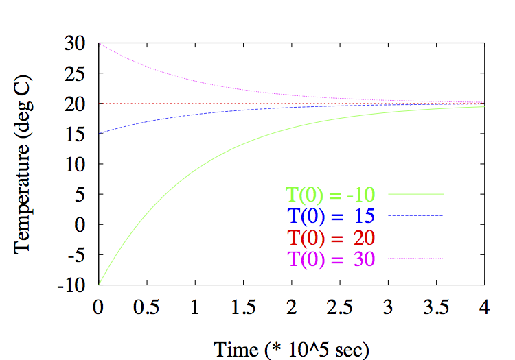
Figure: Conduction Plot of solution curves \(T(t)\) for \(T_0=-10,15,20,30\); parameter values: \(\lambda=10^{-5}\), \(T_a=20\).
Demo: Conduction
Here is an interactive example that investigates the behaviour of the solution.
The first we import the function that does the calculation and plotting. You need to run this cell (how to) to load it. Loading it does not run the function.
[4]:
from numlabs.lab1 import temperature_conduction as tc
You need to call the function. Simpliest call is next cell.
[5]:
# simple call to temperature demo
tc.temperature()
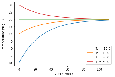
After running as is try changing To = To (the initial temperature), Ta = Ta (the ambient temperature) or la = λ (the effective conductivity) to investigate changes in the solution.
[6]:
# setting different values
# (note this uses the defaults again as written, you should change the values)
tc.temperature(Ta = 20, To = np.array([-10., 10., 20., 30.]), la = 0.00001)

Example Two
Suppose that the rock in the previous example has a \(\lambda\) which is not constant. For example, if that the rock is made of a material whose specific heat varies with the temperature or time, then \(\lambda\) can be a function of \(T\) or \(t\). This might happen if the material composing the rock undergoes a phase transition at a certain critical temperature (for example, a melting ice pellet). The problem is now a non-linear one, for which analytical techniques may or may not provide a solution.
If \(\lambda=\lambda(T)\), a function of temperature only, then the exact solution may be written as
which involves an integral that may or may not be evaluated analytically, in which case we can only approximate the integral. Furthermore, if \(\lambda\) is a function of both \(T\) and \(t\) which is not separable (cannot be written as a product of a function of \(T\) and \(t\)), then we may not be able to write down a closed form for the solution at all, and we must resort to numerical methods to obtain a solution.
Even worse, suppose that we don’t know \(\lambda\) explicitly as a function of temperature, but rather only from experimental measurements of the rock (see Figure Table for an example).
i |
Temperature (\(T_i\)) |
Measured \(\lambda_i\) |
|---|---|---|
0 |
-5.0 |
2.92 |
1 |
-2.0 |
1.59 |
2 |
1.0 |
1.00 |
3 |
4.0 |
2.52 |
4 |
7.0 |
3.66 |
5 |
10.0 |
4.64 |
[7]:
Image(filename="table/table-interp.png",width='60%')
[7]:
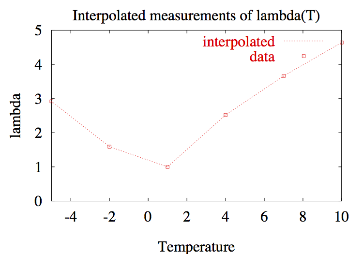
Figure Table: A rock with \(\lambda\) known only at a sequence of discrete temperature values, from experimental measurements. The function \(\lambda(T)\) can be represented approximately using linear interpolation (and the resulting approximate function can then be used to solve the problem numerically.
Then there is no way to express the rock’s temperature as a function, and analytical methods fail us, since we do not know the values at points between the given values. One alternative is to approximate \(\lambda\) at intermediate points by joining successive points with straight lines (this is called linear interpolation), and then use the resulting function in a numerical scheme for computing the solution.
As the above example demonstrates, even for a simple ODE such as 1-d conduction, there are situations where analytical methods are inadequate.
Partial Differential Equations
Example Three
The rock in Example One was considered to be small enough that the effects of heat diffusion in the interior were negligible in comparison to the heat lost by conduction through its surface. In this example, consider a rock that is not small, and whose temperature changes are dominated by internal diffusion effects. Therefore, it is no longer possible to ignore the spatial dependence in the problem.
For simplicity, we will add spatial dependence in one direction only, which corresponds to a “one-dimensional rock”, or a thin rod. Assume that the rod is insulated along its sides, so that heat flows only along its length, and possibly out the ends (see Figure Rod).
[8]:
Image(filename='conduction/rod.png',width='60%')
[8]:
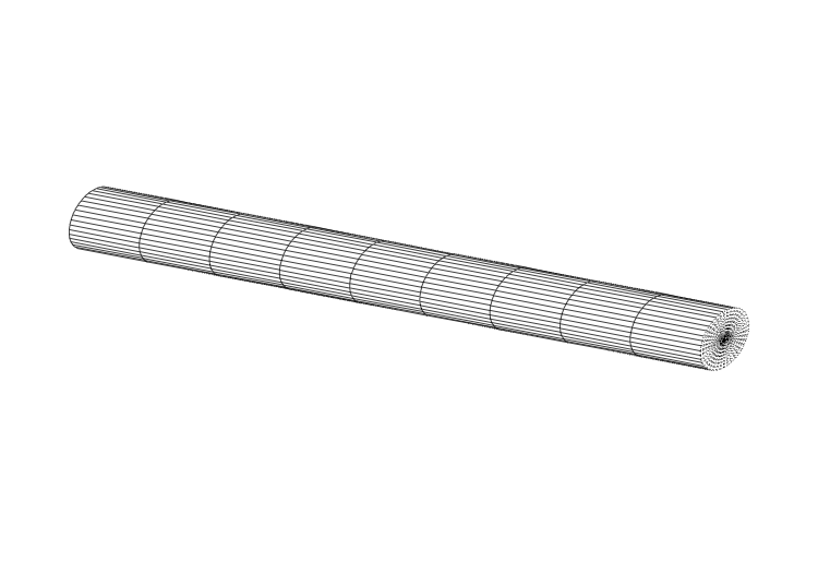
Figure Rod: A thin rod can be thought of as a model for a one-dimensional rock.
Consequently, the temperature varies only with position, \(x\), and time, \(t\), and can be written as a function \(u(x,t)\). The temperature in the rod is governed by the following PDE
for which we have to provide an initial temperature
and boundary values
where
\(\alpha^2\) is the thermal diffusivity of the material,
\(u_0(x)\) is the initial temperature distribution in the rod, and
the boundary conditions indicate that the ends of the rod are held at constant temperature, which we’ve assumed is zero.
Thermal diffusivity is a quantity that depends only on the material from which the bar is made. It is defined by
where \(\kappa\) is the thermal conductivity, \(\rho\) is the density, and \(c\) is the specific heat. A typical value of the thermal diffusivity for a granite bar is \(0.011\;cm^2/sec\), and \(0.0038\;cm^2/sec\) for a bar made of brick.
Using the method of separation of variables, we can look for a temperature function of the form \(u(x,t)=X(x) \cdot T(t)\), which leads to the infinite series solution
where the series coefficients are
Mathematical Note: Details of the derivation can be found in any introductory text in PDE’s (for example, Boyce and DiPrima (1986) [p. 549]).
We do manage to obtain an explicit formula for the solution, which can be used to calculate actual values of the solution. However, there are two obvious reasons why this formula is not of much practical use:
The series involves an infinite number of terms (except for very special forms for the initial heat distribution … such as the one shown below). We might be able to truncate the series, since each term decreases exponentially in size, but it is not trivial to decide how many terms to choose in order to get an accurate answer and here we are already entering the realm of numerical approximation.
Each term in the series requires the evaluation of an integral. When these cannot be integrated analytically, we must find some way to approximate the integrals … numerical analysis rears its head once again!
For most physical problems, an analytical expression cannot be obtained, and the exact formula is not of much use.
However, consider a very special case, when the initial temperature distribution is sinusoidal,
For this problem, the infinite series collapses into a single term
Sample solution curves are given in Figure 1d Diffusion.
[9]:
Image(filename='diffusion/diffusion.png',width='60%')
[9]:
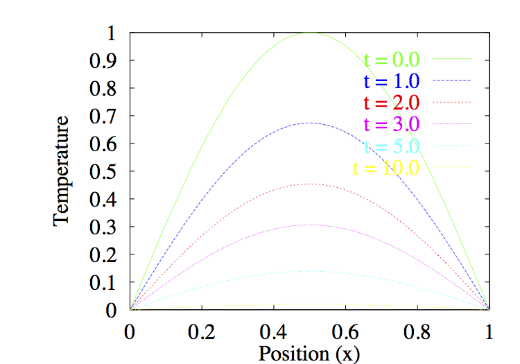
Figure 1d-diffusion Temperature vs. position curves at various times, for heat diffusion in a rod with sinusoidal initial temperature distribution and parameter value \(\alpha=0.2\).
Movie: Diffusion
Here is a movie of the exact solution to the diffusion problem. Run the cell (how to), then run the video. If you want to see the video again, re-run the cell. (The video doesn’t rerun properly from the wysiwyg interface)
[10]:
import IPython.display as display

vid = display.YouTubeVideo("b4D2ktTtw7E", modestbranding=1, rel=0, width=800)
display.display(vid)
Summary
This section is best summed up by the insightful comment of Strang (1986) [p. 587]:
Nature is nonlinear.
Most problems arising in physics (which are non-linear) cannot be solved analytically, or result in expressions that have little practical value, and we must turn to numerical solution techniques.
Discretization
When computing analytical solutions to differential equations, we are dealing with continuous functions; i.e. functions that depend continuously on the independent variables. A computer, however, has only finite storage capacity, and hence there is no way to represent continuous data, except approximately as a sequence of discrete values.
Example Four
We already saw an example of a discrete function in Example Two where the rate function \(\lambda\), depended on the temperature. If \(\lambda\) is not known by some empirical formula, then it can only be determined by experimental measurements at a discrete set of temperature values. In Figure Table, \(\lambda\) is given at a sequence of six temperature points (\((T_i, \lambda_i)\), for \(i = 0, 1, \dots, 5)\)), and so is an example of a discrete function.
The process of interpolation, which was introduced in Example Two, will be considered in more detail next.
Example Five
Consider the two continuous functions
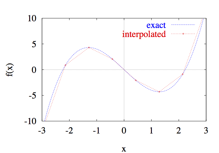
\[f(x)=x^3-5x \;\; {\rm and} \;\; g(x)=x^{2/3} .\](In fact, \(g(x)\) was the function used to generate the values \(\lambda(T)\) in Example Two).
The representation of functions using mathematical notation or graphs is very convenient for mathematicians, where continuous functions make sense. However, a computer has a limited storage capacity, and so it can represent a function only at a finite number of discrete points \((x, y)\).
One question that arises immediately is: What do we do if we have to determine a value of the function which is not at one of the discrete points? The answer to this question is to use some form of interpolation – namely to use an approximation procedure to estimate values of the function at points between the known values.
For example, linear interpolation approximates the function at intermediate points using the straight line segment joining the two neighbouring discrete points. There are other types of interpolation schemes that are more complicated, a few of which are:
quadratic interpolation: every two sucessive points are joined by a quadratic polynomial.
cubic splines: each pair of points is joined by a cubic polynomial so that the function values and first derivatives match at each point.
Fourier series: instead of polynomials, uses a sum of \(\sin nx\) and \(\cos nx\) to approximate the function (Fourier series are useful in analysis, as well as spectral methods).
Chebyshev polynomials: another type of polynomial approximation which is useful for spectral methods.
…many others …
For details on any of these interpolation schemes, see a numerical analysis text such as that by Burden and Faires (1981).
An application of linear interpolation to discrete versions of the functions \(f\) and \(g\) is shown in Figure f and g.
[11]:
Image(filename='discrete/f.png', width='60%')
[11]:
[12]:
Image(filename='discrete/g.png', width='60%')
[12]:
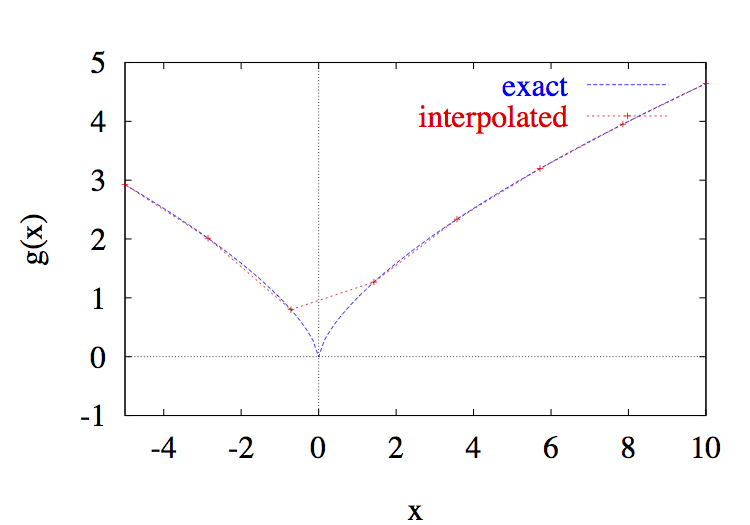
Figure f and g: The functions \(f\) and \(g\) are known only at discrete points. The function can be approximated at other values by linear interpolation, where straight line segments are used to join successive points.
Depending on the function, or number of location of the points chosen, the approximation may be more or less accurate. In Figure f and g, it is not clear which function is approximated more accurately. In the graph of \(f(x)\), the error seems to be fairly small throughout. However, for the function \(g(x)\), the error is large near \(x=0\), and then very small elsewhere. This problem of accuracy of discrete approximations will come up again and again in this course.
Demo: Interpolation
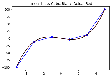
Here is an interactive example demonstrating the use of interpolation (linear and cubic) in approximating functions.
The next cell imports a module containing two python functions that interpolate the two algebraic functions, f and g (Figure f and g). You need to run this cells (how to) to load them.
[13]:
from numlabs.lab1 import interpolate as ip
Once you have loaded the module, you can call the interpolation routines as ip.interpol_f(pn) and ip.interpol_g(pn). pn is the number of points used the interpolation. Watch what changing pn does to the solutions.
[14]:
ip.interpol_f(6)
[14]:
(array([-5., -3., -1.,  1.,  3.,  5.]),
 array([-100.,  -12.,    4.,   -4.,   12.,  100.]))
[15]:
ip.interpol_g(6)
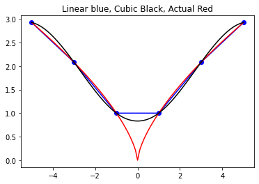
[15]:
(array([-5., -3., -1.,  1.,  3.,  5.]),
 array([2.92401774, 2.08008382, 1.        , 1.        , 2.08008382,
        2.92401774]))
Interpolation Quiz
The accuracy of an approximation using linear or cubic interpolation improves as the number of points is increased. True or False?
In the following, replace ‘xxxx’ by ‘True’, ‘False’, or ‘Hint’
[16]:
print (quiz.interpolation_quiz(answer = 'xxx'))
Acceptable answers are 'True', 'False', or 'Hint'
When solving differential equations numerically, it is essential to reduce the continuous problem to a discrete one. The basic idea is to look for an approximate solution, which is defined at a finite number of discrete points. This set of points is called a grid. Consider the one-dimensional conduction problem of Example One, Conduction, which in its most general form reads
(Conduction Equation)
with initial temperature \(T(0)\).
When we say we want to design a numerical procedure for solving this initial value problem, what we want is a procedure for constructing a sequence of approximations,
defined at a set of discrete \(t\)-points,
Each \(T_i\) is an approximation of the actual temperature at \(t_i\); that is
For now, we will consider equally-spaced points, each of which is separated by a distance \(\Delta t\), so that
An example of such a grid is shown in Figure Grid.
[17]:
Image(filename='discrete/grid.png', width='80%')
[17]:

Figure Grid: A grid of equally-spaced points, \(t_i=t_0+i\Delta t\), for \(i=0,1,2,\ldots\).
This process of reducing a continuous problem to one in a finite number of discrete unknowns is called discretization. The actual mechanics of discretizing differential equations are introduced in the following section.
Discretization Quiz
What phrase best describes “discretization”?
A The development and analysis of methods for the solution of mathematical problems on a computer.
B The process of replacing continuous functions by discrete values.
C Employing the discrete Fourier transform to analyze the stability of a numerical scheme.
D The method by which one can reduce an initial value problem to a set of discrete linear equations that can be solved on a computer.
In the following, replace ‘x’ by ‘A’, ‘B’, ‘C’, ‘D’ or ‘Hint’
[18]:
print (quiz.discretization_quiz(answer = 'x'))
Acceptable answers are 'A', 'B', 'C', 'D' or 'Hint'
Summary
The basic idea in this section is that continuous functions can be approximated by discrete ones, through the process of discretization. In the course of looking at discrete approximations in the interactive example, we introduced the idea of the accuracy of an approximation, and showed that increasing the accuracy of an approximation is not straightforward.
We introduced the notation for approximate solutions to differential equations on a grid of points. The mechanics of discretization as they apply to differential equations, will be investigated further in the remainder of this Lab, as well as in Lab Two.
Difference Approximations to the First Derivative
It only remains to write a discrete version of the differential equation (Conduction Equation) involving the approximations \(T_i\). The way we do this is to approximate the derivatives with finite differences. If this term is new to you, then you can think of it as just another name for a concept you have already seen in calculus. Remember the definition of the derivative of a function :math:`y(t)`, where \(y^\prime(t)\) is written as a limit of a divided difference:
(limit definition of derivative)
We can apply the same idea to approximate the derivative \(dT/dt=T^\prime\) in (Conduction Equation) by the forward difference formula, using the discrete approximations, \(T_i\):
(Forward Difference Formula)
Example Six
In order to understand the ability of the formula (Forward Difference Formula) to approximate the derivative, let’s look at a specific example. Take the function \(y(x)=x^3-5x\), and apply the forward difference formula at the point \(x=1\). The function and its tangent line (the short line segment with slope \(y^\prime(1)\)) are displayed in Figure Tangents.
[19]:
Image(filename='deriv/deriv.png', width='60%')
[19]:
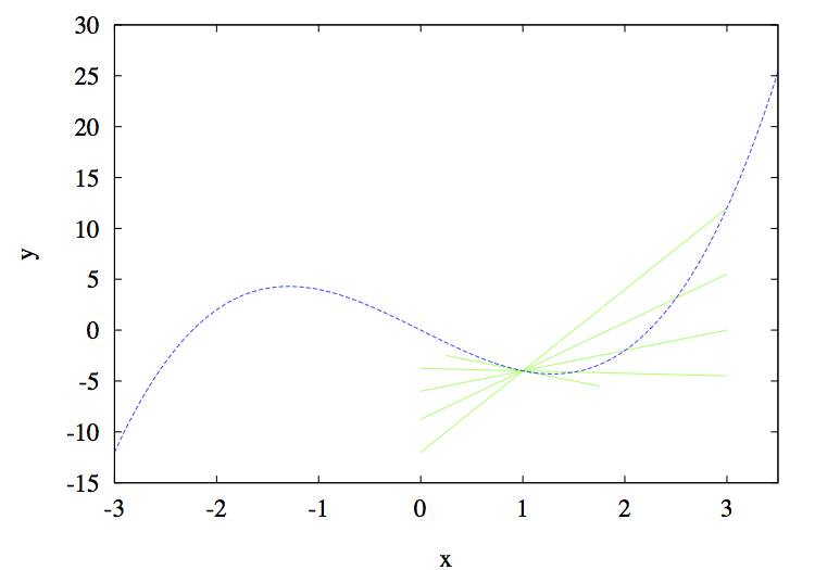
Figure Tangents: Plot of the function \(y=x^3-5x\) and the forward difference approximations to the derivative for various values of \(\Delta t\)
Each of the remaining line segments represents the forward difference approximation to the tangent line for different values of \(\Delta t\), which are simply the secant lines through the points :math:`(t, y(t))` and :math:`(t+Delta t, y(t+Delta t))`. Notice that the approximation improves as \(\Delta t\) is reduced. This motivates the idea that grid refinement improves the accuracy of the discretization …but not always (as we will see in the coming sections).
Investigation
Investigate the use of the forward difference approximation of the derivative in the following interactive example.
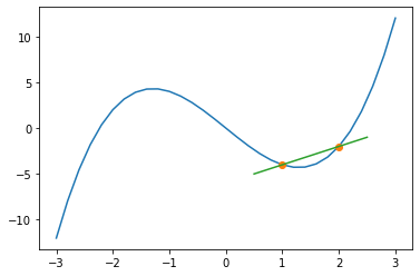
The next cell loads a python function that plots a function f(x) and approximates its derivative at \(x=1\) based on a second x-point that you chose (xb). You need to run this cell (how to) to load it.
[20]:
from numlabs.lab1 import derivative_approx as da
Once you have loaded the function you can call it as da.plot_secant(xb) where xb the second point used to estimate the derivative (slope) at \(x=1\). You can compare the slope of the estimate (straight line) to the slope of the function (blue curve).
[21]:
da.plot_secant(2.)
Forward Euler Method
We can now write down a discrete version of our model ODE problem (Conduction Equation) at any point \(t_i\) by
discretizing the derivative on the left hand side (for example, using the forward difference approximation (Forward Difference Formula);
evaluating the right hand side function at the discrete point \(t_i\).
The discrete form of the problem is
or, after rearranging,
This formula is called the Forward Euler method (since it uses forward differences). Notice that this formula relates each discrete solution value to the solution at the preceding \(t\)-point. Consequently, if we are given an initial value \(T(0)\), then all subsequent values of the solution are easily computed.
(Note: The forward Euler formula for the more general first-order IVP in (Model ODE) is simply \(y_{i+1} = y_i + \Delta t f(y_i,t_i)\).)
Example Seven
Let us now turn to another example in atmospheric physics to illustrate the use of the forward Euler method. Consider the process of condensation and evaporation in a cloud. The saturation ratio, \(S\), is the ratio of the vapour pressure to the vapour pressure of a plane surface of water at temperature \(T\). \(S\) varies in time according to the
(saturation development equation)
\[\frac{dS}{dt} = \alpha S^2 + \beta S + \gamma,\]where \(\alpha\), \(\beta\) and \(\gamma\) are complicated (but constant) expressions involving the physical parameters in the problem (and so we won’t reproduce them here).
What are some physically reasonable values of the parameters (other than simply \(\alpha<0\) and \(\gamma>0\))?
Chen (1994) gives a detailed derivation of the equation, which is a non-linear, first order ODE (i.e. non-linear in the dependent variable \(S\), and it contains only a first derivative in the time variable). Chen also derives an analytical solution to the problem which takes a couple pages of messy algebra to come to. Rather than show these details, we would like to use the forward Euler method in order to compute the solution numerically, and as we will see, this is actually quite simple.
Using the (forward difference formula), the discrete form of the (saturation development equation) is
\[S_{i+1} = S_i + \Delta t \left( \alpha S_i^2 + \beta S_i + \gamma \right).\]Consider an initial saturation ratio of \(0.98\), and take parameter values \(\alpha=-1\), \(\beta=1\) and \(\gamma=1\). The resulting solution, for various values of the time step \(\Delta t\),is plotted in Figure Saturation Time Series.
[22]:
Image(filename='feuler/sat2.png', width='60%')
[22]:
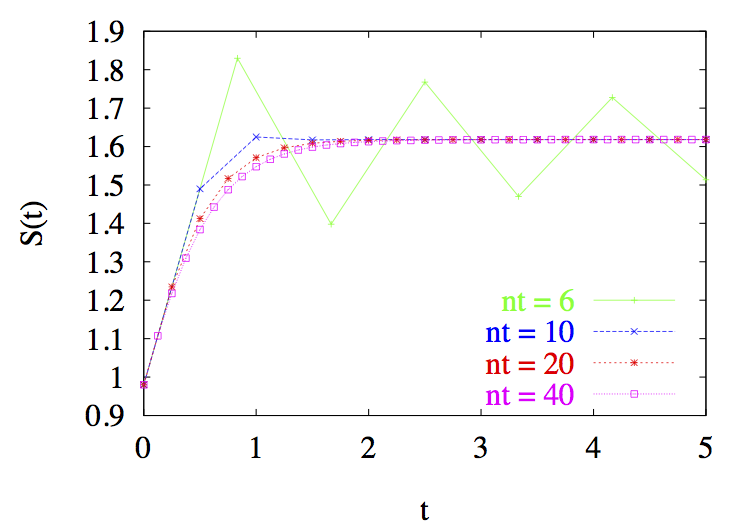
Figure Saturation Time Series: Plot of the saturation ratio as a function of time using the Forward Euler method. “nt” is the number of time steps.
There are two things to notice here, both related to the importance of the choice of time step \(\Delta t\):
As \(\Delta t\) is reduced, the solution appears to converge to one solution curve, which we would hope is the exact solution to the differential equation. An important question to ask is: When will the numerical method converge to the exact solution as :math:`Delta t` is reduced?
If \(\Delta t\) is taken too large, however, the numerical solution breaks down. In the above example, the oscillations that occur for the largest time step (when \(nt=6\)) are a sign of numerical instability. The differential problem is stable and exhibits no such behaviour, but the numerical scheme we have used has introduced an instability. An obvious question that arises is: How can we avoid introducing instabilities in a numerical scheme?
Neither question has an obvious answer, and both issues will be investigated further in Lab 2.
Other Approximations
Look again at the (limit definition of derivative), and notice that an equivalent expression for \(T^\prime\) is
From this, we can derive the backward difference formula for the first derivative,
(Backward Difference Formula)
and similarly the centered difference formula
(Centered Difference Formula)
The corresponding limit formulas are equivalent from a mathemtaical standpoint, but the discrete formulas are not! In particular, teh accuracy and stability of numerical schemes derived from the three difference formulas: (Forward Difference Formula), (Backward Difference Formula) and (Centered Difference Formula) are quite different. More will said on this in the next Lab.
Summary
This section introduces the use of the forward difference formula to discretize the derivatives in a first order differential equation. The resulting numerical scheme is called the forward Euler method. We also introduced the backward and centered difference formulas for the first derivative, which were also obtained from the definition of derivative.
You saw how the choice of grid spacing affected the accuracy of the solution, and were introduced to the concepts of convergence and stability of a numerical scheme. More will be said about these topics in the succeeding lab, as well as other methods for discretizing derivatives.
Generalizations
The idea of discretization introduced in the previous section can be generalized in several ways, some of which are:
problems with higher derivatives,
systems of ordinary differential equations,
boundary value problems, and
partial differential equations.
Higher Derivatives
Many problems in physics involve derivatives of second order and higher. Discretization of these derivatives is no more difficult than the first derivative in the previous section. The difference formula for the second derivative, which will be derived in Lab #2, is given by
(Centered Second Derivative)
and is called the second-order centered difference formula for the second derivative (“centered”, because it involves the three points centered about \(t_i\), and “second-order” for reasons we will see in the next Lab). We will apply this formula in the following example …
Example Eight
A weather balloon, filled with helium, climbs vertically until it reaches its level of neutral buoyancy, at which point it begins to oscillate about this equilibrium height. We can derive a DE describing the motion of the balloon by applying Newton’s second law:
where
\(y(t)\) is the displacement of the balloon vertically from its equilibrium level, \(y=0\);
\(m\) is the mass of the balloon and payload;
the oscillations are assumed small, so that we can assume a linear functional form for the buoyant force, \(-\gamma y\).
This problem also requires initial values for both the initial displacement and velocity:
[23]:
Image(filename='balloon/balloon.png', width='60%')
[23]:
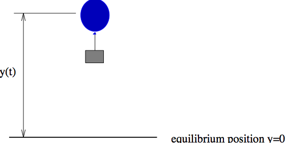
Figure Weather Balloon: A weather balloon oscillating about its level of neutral buoyancy.
Problem One
Using the centered difference formula (Centered Second Derivative) for the second derivative, and the forward difference formula (Forward Difference Formula) for the first derivative at the point \(t_i\), derive a difference scheme for \(y_{i+1}\), the vertical displacement of the weather balloon.
What is the difference between this scheme and the forward Euler scheme from [Example Seven](#Example-Seven] , Fix Link related to the initial conditions? (Hint: think about starting values …)
Given the initial values above, explain how to start the numerical integration.
Note: There are a number of problems in the text of each lab. See the syllabus for which problems you are assigned as part of your course. That is, you don’t have to do them all!
Systems of First-order ODE’s
Discretization extends in a simple way to first-order systems of ODE’s, which arise in many problems, as we will see in some of the later labs. For now, though, we can see:
Example 9
The second order DE for the weather balloon problem from Example Eight can be rewritten by letting \(u=dy/dt\). Then,
\begin{align} \frac{dy}{dt} &= u\\ \frac{du}{dt} &= -\frac{\beta}{m} u - \frac{\gamma}{m} y \end{align}
which is a system of first order ODE’s in \(u\) and \(y\). This set of differential equations can be discretized to obtain another numerical scheme for the weather balloon problem.
Problem Two
Derive a difference scheme for the problem based on the above system of two ODE’s using the forward difference formula for the first derivative.
By combining the discretized equations into one equation for y, show that the difference between this scheme and the scheme obtained in problem one is the difference formula for the second derivative.
Boundary Value Problem
So far, we’ve been dealing with initial value problems or IVP’s (such as the problem of heat conduction in a rock in Example One): a differential equation is given for an unknown function, along with its initial value. There is another class of problems, called boundary value problems (or BVP’s), where the independent variables are restricted to a closed domain (as opposed to an open domain) and the solution (or its derivative) is specified at every point along the boundary of the domain. Contrast this to initial value problems, where the solution is not given at the end time.
A simple example of a boundary value problem is the steady state heat diffusion equation problem for the rod in Example Three. By steady state, we mean simply that the rod has reached a state where its temperature no longer changes in time; that is, \(\partial u/\partial t = 0\). The corresponding problem has a temperature, \(u(x)\), that depends on position only, and obeys the following equation and boundary conditions:
This problem is known as an initial-boundary value problem(or IBVP), since it has a mix of both initial and boundary values.
The structure of initial and boundary value problems are quite different mathematically: IVP’s involve a time variable which is unknown at the end time of the integration (and hence the solution is known on an open domain or interval), whereas BVP’s specify the solution value on a closed domain or interval. The numerical methods corresponding to these problems are also quite different, and this can be best illustrated by an example.
Example 10
We can discretize the steady state diffusion equation using the centered difference formula for the second derivative to obtain:
where \(u_i\approx u(i/N)\) and \(i=0,1,\ldots,N\) (and the factor of \((\Delta x)^2 = {1}/{N^2}\) has been multiplied out). The boundary values \(u_0\) and \(u_N\) are both known to be zero, so the above expression represents a system of \(N-1\) equations in \(N-1\) unknown values \(u_i\) that must be solved for simultaneously. The solution of such systems of linear equations will be covered in more detail in Lab #3 in fact, this equation forms the basis for a Problem in the Linear Algebra Lab.
Compare this to the initial value problems discretized using the forward Euler method, where the resulting numerical scheme is a step-by-step, marching process (that is, the solution at one grid point can be computed using an explicit formula using only the value at the previous grid point).
Partial Differential Equations
So far, the examples have been confined to ordinary differential equations, but the procedure we’ve set out for ODE’s extends with only minor modifications to problems involving PDE’s.
Example 11
To illustrate the process, let us go back to the heat diffusion problem from Example Three, an initial-boundary value problem in the temperature \(u(x,t)\):
along with initial values
and boundary values
As for ODE’s, the steps in the process of discretization remain the same:
First, replace the independent variables by discrete values
\[x_i = i \Delta x = \frac{i}{M}, \;\; \mbox{where $i=0, 1, \ldots, M$, and}\]\[t_n = n \Delta t, \;\; \mbox{where $n=0, 1, \ldots$}\]In this example, the set of discrete points define a two-dimensional grid of points, as pictured in Figure PDE Grid.
[24]:
Image(filename='pdes/pde-grid.png', width='40%')
[24]:
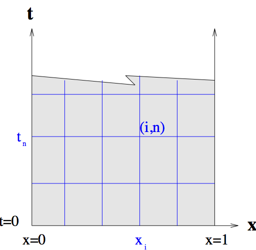
Figure PDE Grid: The computational grid for the heat diffusion problem, with discrete points \((x_i,t_n)\).
Replace the dependent variables (in this example, just the temperature \(u(x,t)\)) with approximations defined at the grid points:
\[U_i^n \approx u(x_i,t_n).\]The boundary and initial values for the discrete temperatures can then be written in terms of the given information.
Approximate all of the derivatives appearing in the problem with finite difference approximations. If we use the centered difference approximation (Centered Second Derivative) for the second derivative in \(x\), and the forward difference formula (Forward Difference Formula) for the time derivative (while evaluating the terms on the right hand side at the previous time level), we obtain the following numerical scheme: :nbsphinx-math:`begin{equation}
- U_i^{n+1} = U_i^n + frac{alpha^2 Delta t}{(Delta x)^2} left(
U_{i+1}^n - 2 U_i^n + U_{i-1}^n right)
end{equation}`
Given the initial values, \(U_i^0=u_0(x_i)\), and boundary values \(U_0^n=U_M^n=0\), this difference formula allows us to compute values of temperature at any time, based on values at the previous time.
There are, of course, other ways of discretizing this problem, but the above is one of the simplest.
Mathematical Notes
Solution to the Heat Conduction Equation
In Example One, we had the equation
subject to the initial condition \(T(0)\). This equation can be solved by separation of variables, whereby all expressions involving the independent variable \(t\) are moved to the right hand side, and all those involving the dependent variable \(T\) are moved to the left
The resulting expression is integrated from time \(0\) to \(t\)
(where \(s\) and \(S\) are dummy variables of integration), which then leads to the relationship
or, after exponentiating both sides and rearranging,
which is exactly the Conduction Solution equation.
References
Boyce, W. E. and R. C. DiPrima, 1986: Elementary Differential Equations and Boundary Value Problems. John Wiley & Sons, New York, NY, 4th edition.
Burden, R. L. and J. D. Faires, 1981: Numerical Analysis. PWS-Kent, Boston, 4th edition.
Chen, J.-P., 1994: Predictions of saturation ratio for cloud microphysical models. Journal of the Atmospheric Sciences, 51(10), 1332–1338.
Garcia, A. L., 1994: Numerical Methods for Physics. Prentice-Hall, Englewood Cliffs, NJ.
Strang, G., 1986: Introduction to Applied Mathematics. Wellesley-Cambridge Press, Wellesley, MA.
Glossary
backward difference discretization: used to estimate a derivative – uses the current points and points with smaller independent variable.
boundary value problem: a differential equation (or set of differential equations) along with boundary values for the unknown functions. Abbreviated BVP.
BVP: see boundary value problem
centre difference discretization: used to estimate a derivative – uses a discretization symmetric (in independent variable) around the current point.
closed domain: a domain for which the value of the dependent variables is known on the boundary of the domain.
converge: as the discretization step (eg. ∆t) is reduced the solutions generated approach one solution curve.
DE: see differential equation
dependent variable: a variable which is a (possibly unknown) function of the independent variables in a problem; for example, in a fluid the pressure can be thought of as a dependent variable, which depends on the time t and position (x, y, z).
differential equation: an equation involving derivatives. Abbreviated DE.
discretization: when referring to DE’s, it is the process whereby the independent variables are replaced by a grid of discrete points; the dependent variables are replaced by approximations at the grid points; and the derivatives appearing in the problem are replaced by a finite difference approximation. The discretization process replaces the DE (or DE’s) with an algebraic equation or finite system of algebraic equations which can be solved on a computer.
finite difference: an approximation of the derivative of a function by a difference quotient involving values of the function at discrete points. The simplest method of deriving finite difference formulae is using Taylor series.
first order differential equation: a differential equation involving only first derivatives of the unknown functions.
forward difference discretization: used to calculate a derivative – uses the current points and points with larger independent variable.
grid: when referring to discretization of a DE, a grid is a set of discrete values of the independent variables, defining a mesh or array of points, at which the solution is approximated.
independent variable: a variable that does not depend on other quantities (typical examples are time, position, etc.)
initial value problem: a differential equation (or set of differential equations) along with initial values for the unknown functions. Abbreviated IVP.
interpolation: a method for estimating the value of a function at points intermediate to those where its values are known.
IVP: initial value problem
linear: pertaining to a function or expression in which the quantities appear in a linear combination. If \(x_i\) are the variable quantities, and \(c_i\) are constants, then any linear function of the \(x_i\) can be written in the form \(c_0 + \sum_i c_i \cdot x_i\).
linear interpolation: interpolation using straight lines between the known points
Navier-Stokes equations: the system of non-linear PDE’s that describe the time evolution of the flow of a fluid.
non-linear: pertaining to a function or expression in which the quantities appear in a non-linear combination.
numerical instability: although the continuous differential equation has a finite solution, the numerical solution grows without bound as the numerical interation proceeds.
ODE: see ordinary differential equation
open domain: a domain for which the value of one or more dependent variables is unknown on a portion of the boundary of the domain or a domain for which one boundary (say time very large) is not specified.
ordinary differential equation: a differential equation where the derivatives appear only with respect to one independent variable. Abbreviated ODE.
partial differential equation: a differential equation where derivatives appear with respect to more than one independent variable. Abbreviated PDE.
PDE: see partial differential equation
second order differential equation: a differential equation involving only first and second derivatives of the unknown functions.
separation of variables: a technique whereby a function with several dependent variables is written as a product of several functions, each of which depends on only one of the dependent variables. For example, a function of three unknowns, u(x, y, t), might be written as u(x, y, t) = X(x) · Y (y) · T (t).
[ ]: